https://ift.tt/VZu2zQg Artificial Intelligence in Healthcare Part III Written by Sandra Carrasco and Sylwia Majchrowska . Figure 1. E...
Artificial Intelligence in Healthcare Part III
Written by Sandra Carrasco and Sylwia Majchrowska.
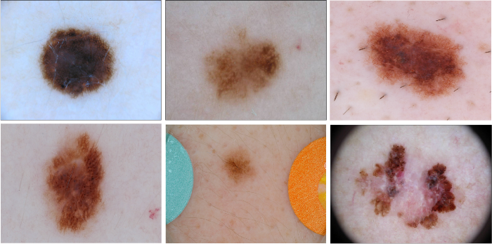
The use of healthcare data in the development of deep learning models is associated with challenges related to personal data and regulatory issues. Patient data cannot be freely shared and is therefore limited in its usefulness for creating AI solutions. In our previous post we discussed the potential of synthetic data in Healthcare. We described studies on the open-source International Skin Imaging Collaboration (ISIC) archive [1], which is one of the biggest (and highly unbalanced) datasets of dermatoscopic images of skin lesions. We chose the StyleGAN2-ADA architecture in a conditional setting to generate images from both melanomas and non-melanomas. Today we want to introduce you to the topic of evaluation of the GAN-generated synthetic data.
Evaluation of GANs
There is no objective loss function used to train the generator of a GAN, and therefore, no way to objectively assess the progress of the training and the relative or absolute quality of the model from loss alone. Instead, a suite of qualitative and quantitative techniques have been developed to assess the performance of a GAN model based on the quality and diversity of the generated synthetic images. For a thorough survey, see the article Pros and Cons of GAN Evaluation Measures [2].
Qualitative
Since there is no objective loss function used when training generative models, these must be evaluated using the quality of the generated synthetic images. One of the most basic and useful ways to evaluate your GAN is by manually inspecting and judging the generated examples from different iteration steps.
However, this has many limitations:
- It is subjective and includes the biases of the reviewer.
- It requires domain knowledge to tell what is realistic and what is not. In our specific case, it is extremely important to count on the aid of dermatologists who can assess the fake examples.
- It is limited in terms of the number of images that can be reviewed.
No clear best practice has emerged on how, precisely, one should qualitatively review the generated images as it is likely to vary a lot from case to case. Therefore, we will not explore this topic in detail in this post.
Quantitative
In this section, we will inspect some metrics that are generally used to evaluate generative models during training. These can be combined with qualitative assessment to provide a robust assessment of GAN models.
When measuring how well our GAN performs we need to evaluate two main properties:
- Fidelity: the quality of the generated samples. Measures how realistic the images are. You can think of it as how different each fake sample is from its nearest real sample.
- Diversity: the variety of the generated samples. Measures how well the generated images cover the whole diversity or variety of the real distribution.

By capturing fidelity and diversity, you can get a pretty good notion of how well your generator is generating fake images. However, there is another dimension that we need to evaluate in order to assess our generative model.
- Authenticity/Generalizability: it measures the rate at which the model invents new samples and try to spot overfitting to the real data. Alaa et al. [5] define it as the fraction of generated samples that are closer to the training data set than other training data points.
Finally, synthetic data should be just as useful as real data for the subsequent task when used for the same predictive purposes.
- Predictive performance: we train on synthetic data and test on real data. This evaluates how well the synthetic data covers the distribution of the real data. We can also train and test models with synthetic data. This would allow us to evaluate whether synthetic data preserves the ranking of the predictive models on the real data.
We will now discuss the introduced quantitative methods in more detail.
Commonly computed metrics
The most common metrics to evaluate GAN performance are Fréchet Inception Distance (FID) and Kernel Inception Distance (KID). They evaluate fidelity (quality of images) and diversity (variety of images).
Fréchet Inception Distance (FID)
In order to compare real and fake images, classifiers can be used as feature extractors. The most commonly used feature extractor is the Inception-v3 classifier, which is pre-trained on ImageNet. Cutting off the output layer, we can get the embeddings of real and fake images to extract the feature distance. These embeddings are two multivariate normal distributions, which can be compared using the Multivariate Normal Fréchet Distance or Wasserstein-2 distance. However, the FID score has some shortcomings. First, it uses a pre-trained Inception model, which may not capture all features. Secondly, it needs a large sample size. Finally, it’s slow to run and uses limited statistics (only mean and covariance).
Kernel Inception Distance (KID)
KID has been proposed as a replacement for FID. FID has no unbiased estimator which leads to higher expected value on smaller datasets. KID is suitable for smaller datasets since its expected value does not depend on the number of samples. It is also computationally lighter, more numerically stable and simpler to implement.
Inception Score
Similar to FID and KID, this score measures both the diversity and fidelity of the images. The higher it is, the more real and diverse the generated images are
The inception score is calculated by first using a pre-trained Inception v3 model to predict the class probabilities for each generated image. These are conditional probabilities, e.g. class labels conditional on the generated image. Images that are classified strongly as one class over all other classes indicate a high quality. As such, if the image contains a realistic thing, the conditional probabilities follow a narrow distribution (low entropy).
Secondly, we use the marginal probability. This is the label probability distribution of all generated images. Therefore, it tells us how much variety there is in our generated images. Hence, we would prefer the integral of the marginal probability distribution to have a high entropy, i.e. our generator to synthesize as many different classes as possible.
These elements are combined by calculating the Kullback-Leibler divergence, or KL divergence (relative entropy), between the conditional and marginal probability distributions. If it is high, our distributions are dissimilar, i.e. each image has a clear label, and all images are collectively varied.
This score has several limitations. First, it only looks at the fake images, without comparing them to the real ones. Same as with FID, it is limited by what the Inception classifier can detect, which is directly linked to the training data. In general, it tries to capture fidelity and diversity as well, but it performs worse than FID. If you want to know more, go to this fantastic post by David Mack on A simple explanation of the Inception Score.
Precision and Recall
Another type of metrics, so known for classification and detection tasks, are precision and recall. We can define them as:
- Precision relates to fidelity. It looks at overlap between real and fake data over how many non-realistic images the generator produces (non-overlap red).
- Recall relates to diversity. It looks at overlap between reals and fakes, over all the reals that the generator cannot model (non-overlap blue).
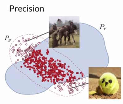
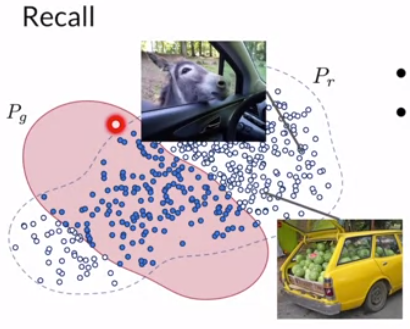
The problem with precision-recall is that it can have a perfect precision score but poor generative distribution because it only generates outliers in the real distribution. Additionally, we cannot detect mode collapse or mode invention.
Perceptual Path Length
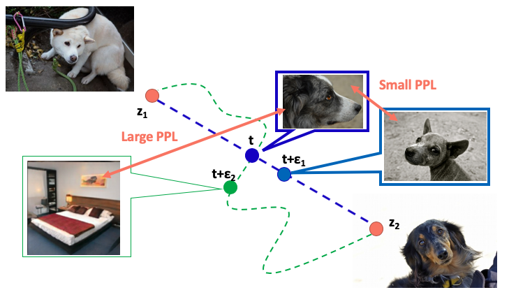
Another important metric to assess Generative networks is the Perceptual Path Length (PPL). It is a measure of feature disentanglement, a type of regularization that encourages good conditioning in the mapping from latent codes to images. Before we discuss PPL further, let us discuss the latent space.
StyleGAN2 Latent Space: In StyleGAN we find two latent spaces, the z-space and the w-space. First, the Z-space is where z-vectors which come from a Gaussian distribution, reside. In a standard GAN, a z-vector is directly fed into a generator to generate a fake image. In styleGAN, however, this vector is passed through a mapping network to produce a w-vector or a style vector. The W space does not follow any specific distribution, but it is learnt during training so that it can better model the underlying distribution of the real data. The w-vector is then fed into the synthesis network at various layers for the final generation. Both Z and W spaces are 512 dimensional. The latent space W is the key to controlling the attributes of an image since it is disentangled, meaning each of the 512 dimensions encodes unique information about the image.
The aim of PPL is to establish that the mapping from the latent space to image space is well-conditioned. This is done by encouraging that a fixed-size step in the latent W-space results in a non-zero, fixed-magnitude change in the image. We can measure the deviation from this ideal empirically by stepping into random directions in the image space and observing the corresponding w gradients. These gradients should have close to an equal length regardless of w or the image-space direction.
This leads to more reliable and consistently behaving models, making architecture exploration easier. It is also observed that the smoother generator is significantly easier to invert.
Projection into the latent space
In order to further explore and understand our generative network, we can project the real images to the latent space. This basically means that you want to get the w latent code (512 numbers) that will cause the generator to make an output that looks like our image.
With GANs we don’t have a direct way to extract latent codes from input images, but we can optimize for it in the following way:
- Generate an output from a starting latent vector.
- Feed the target image and the generated image to a VGG16 model that acts as a feature extractor.
- Take the features from both images, compute the loss on the difference between them and do backpropagation.
We projected half the images from the training dataset for two reasons:
- To spot data leakage, i.e. assess overfitting.
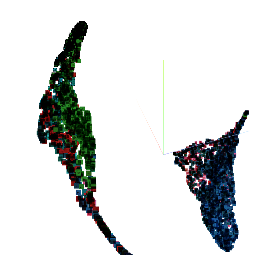
- To visualize the projected latent codes in a 3D space and study the distribution, try to find clusters and study the edge cases.
Evaluating authenticity and overfitting
How can we assess the generalization ability or authenticity of our model? In other words, how do we ensure that our model does not simply copy the data it has been trained on? This is an essential concept to ensure a truly generative model.
However, this is an open question in the field [5, 6]. We tried a simplistic approach. To measure the authenticity and ensure that our generative model is not copying the real data we performed the following experiment.
First, we projected 12 thousand samples from the real dataset into the latent space of the generator. This gave us the latent codes that caused our generator to synthesize the most similar output to the input image. To optimize for a latent code for the given input images, we used a VGG16 model as a feature extractor and computed the loss on the difference of the extracted features for both the target image and generated output and performed backpropagation.
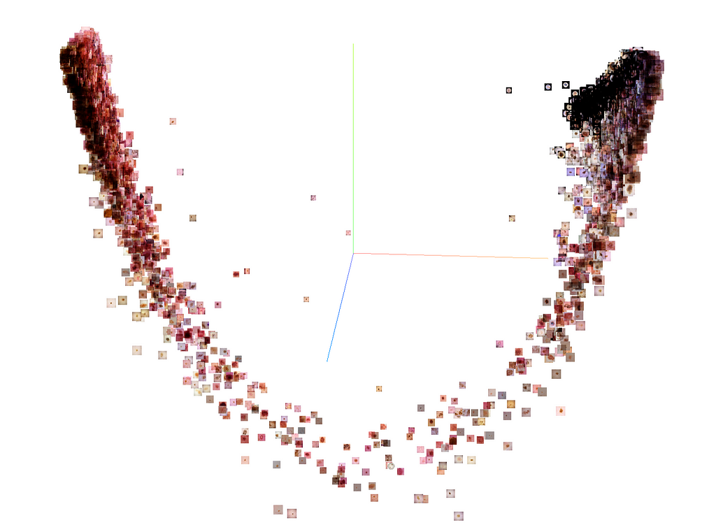
Next, we extracted the features of both the real and their projected images using the last convolutional layer of our classifier trained on real and synthetic data. These embeddings were visualized in a 3D space using t-distributed stochastic neighbor embedding (t-SNE).
This allows visually exploring the closest near neighbors of each real image using cosine distances, and in this way examining how close the real images and their corresponding generated images are.
We treated this as a measure of the authenticity of the generated samples. We spotted that some of the images (which proves their authenticity) were very distant from their projections but still resembled the target image (which proves their fidelity).
Solving the subsequent task
Generating artificial data is not an end in itself, in fact it is the process of creating a tool for another tool. Predictive performance, or solving a subsequent task, can assess the validity of our synthetic data. In our research we used synthetic images of moles to balance the ISIC dataset, which means adding several thousand synthetic images of melanoma. As we mentioned before synthetic data should be just as useful as real data when used for the same predictive purposes. For our binary classification task we used artificial data in a few scenarios:
- balancing the real training subset by adding only synthetic melanoma samples and testing on the real validation subset,
- balancing the real training subset by adding synthetic images belonging to both classes and testing on the real validation subset,
- using a large amount of synthetic training subset (with the same amount of data per each class) and testing on a real validation subset.
The best results were achieved for mixing real and synthetic images of melanomas in a balanced training subset. The calculated accuracy is very close to the accuracy achieved only for real samples which can prove the serviceability of artificial data.
Regardless of how useful the synthetic data would be, we found that all the artifacts, like black frames or medical rulers, found in the real data are reflected also in the artificial. But this is material for another story…
To reproduce the described study we encourage you to check out our github repository and read more about our research in the provided README file.
GitHub - aidotse/stylegan2-ada-pytorch: StyleGAN2-ADA for generation of synthetic skin lesions
In this other post we show how to prepare your data using SIIM-ISIC 2020 dataset and StyleGAN2 for synthetic image generation of skin lesions.
Literature
- ISIC Archive
- Pros and Cons of GAN Evaluation Measures
- An empirical study on evaluation metrics of generative adversarial networks
- Generative Adversarial Networks (GANs) Specialization
- How Faithful is your Synthetic Data? Sample-level Metrics for Evaluating and Auditing Generative Models
- A Non-Parametric Test to Detect Data-Copying in Generative Mode
On the evaluation of Generative Adversarial Networks was originally published in Towards Data Science on Medium, where people are continuing the conversation by highlighting and responding to this story.
from Towards Data Science - Medium https://ift.tt/Z5pPouy
via RiYo Analytics

No comments