https://ift.tt/cebHQWG If you've ever wondered whether learning Rust is worth the effort, or whether working remotely actually pays mo...
If you've ever wondered whether learning Rust is worth the effort, or whether working remotely actually pays more, you're not alone. These are the kinds of questions that sound impossible to answer objectively, but with the right dataset and the right tools, they become exactly the kind of problem machine learning was built for.
In this project walkthrough, we're going to use the 2023 Stack Overflow Developer Survey to build a machine learning model that predicts tech salaries. With over 80,000 developer responses from around the world, it's one of the most comprehensive datasets on what people in our industry actually earn, and what might be driving those earnings.
Part 1 focuses entirely on the data preparation side of the pipeline: cleaning messy survey responses, handling missing values, encoding categorical variables, and engineering features that a model can actually work with. It's a lot of work, but it's also where the most important decisions in any ML project get made.
What You'll Learn
By the end of Part 1, you'll know how to:
- Clean and prepare large-scale survey data for ML modeling
- Handle missing data and make informed decisions about imputation vs. dropping
- Filter outliers and assess data quality in a real-world dataset
- Encode survey responses, including multi-select skills, ordinal rankings, and experience levels
- Avoid data leakage during preprocessing
- Apply real-world tradeoffs in preprocessing decisions
Before You Start
To follow along effectively, make sure you have:
- Intermediate Python and pandas skills
- Some familiarity with the machine learning workflow
- Basic experience with exploratory data analysis (EDA)
You'll also want these libraries installed: pandas, scikit-learn, matplotlib, and seaborn.
You can access the project in the Dataquest app here, and find the dataset on the Stack Overflow 2023 Developer Survey Kaggle page. The full solution notebook is available on GitHub.
The Dataset
Stack Overflow runs an annual survey of the people who use their platform, and the result is a fascinating snapshot of the global developer community. We're using the 2023 edition, which includes responses from nearly 90,000 developers covering everything from what languages they use to how they feel about AI.
Our goal is to predict ConvertedCompYearly, which is each respondent's annual compensation normalized to U.S. dollars. This is our target variable, and it's what we'll be trying to predict in Part 2.
One important note: we're working with a slimmed-down version of the dataset. The original includes almost 90,000 rows and many more columns, but we've removed rows where the target variable was null, and dropped columns unrelated to salary prediction (like how often someone uses Stack Overflow, or what technologies they want to work with but haven't yet). If you download the full dataset directly from Kaggle, you'll need to do some additional cleaning before following along.
Let's start by loading our libraries and reading in the data.
import pandas as pd
import numpy as np
import matplotlib.pyplot as plt
import seaborn as sns
from sklearn.model_selection import train_test_split
from sklearn.linear_model import LinearRegression
from sklearn.metrics import mean_squared_error, r2_score, mean_absolute_error

df = pd.read_csv('survey_results_slim.csv')
df.info()
<class 'pandas.core.frame.DataFrame'>
RangeIndex: 48019 entries, 0 to 48018
Data columns (total 33 columns):
# Column Non-Null Count Dtype
--- ------ -------------- -----
0 MainBranch 48019 non-null object
1 Age 48019 non-null object
2 Employment 48007 non-null object
3 RemoteWork 47940 non-null object
4 EdLevel 48019 non-null object
5 LearnCode 47935 non-null object
6 LearnCodeOnline 38414 non-null object
7 YearsCode 47950 non-null object
8 YearsCodePro 47825 non-null object
9 DevType 47904 non-null object
10 OrgSize 47982 non-null object
11 Country 48019 non-null object
12 LanguageHaveWorkedWith 47883 non-null object
13 DatabaseHaveWorkedWith 41764 non-null object
14 PlatformHaveWorkedWith 37375 non-null object
15 WebframeHaveWorkedWith 37865 non-null object
16 MiscTechHaveWorkedWith 31769 non-null object
17 ToolsTechHaveWorkedWith 44055 non-null object
18 NEWCollabToolsHaveWorkedWith 47435 non-null object
19 OpSysPersonal use 47534 non-null object
20 OpSysProfessional use 45030 non-null object
21 OfficeStackAsyncHaveWorkedWith 41999 non-null object
22 OfficeStackSyncHaveWorkedWith 47015 non-null object
23 AISearchHaveWorkedWith 29485 non-null object
24 AIDevHaveWorkedWith 13940 non-null object
25 AISelect 48019 non-null object
26 AIToolCurrently Using 19550 non-null object
27 TBranch 46156 non-null object
28 ICorPM 32639 non-null object
29 WorkExp 32638 non-null float64
30 ProfessionalTech 31726 non-null object
31 Industry 27747 non-null object
32 ConvertedCompYearly 48019 non-null float64
dtypes: float64(2), object(31)We've got 48,019 rows and 33 columns, and right away we can see something that's going to shape a lot of our decisions: almost every column is an object type. Machine learning models need numbers to work with, so a significant portion of what we're about to do is figuring out how to convert all of these string values into something numeric and meaningful.
Step 1: Dropping Columns with Too Much Missing Data
Before we tackle data types, let's see which columns are missing so much data that they're not worth keeping.
missing_pct = (df.isnull().sum() / len(df) * 100).sort_values(ascending=False)
print("Missing data percentage:\n", missing_pct[missing_pct > 50])
print("\nTotal columns with more than 50% missing data:", (missing_pct > 50).sum())
Missing data percentage:
AIDevHaveWorkedWith 70.969824
AIToolCurrently Using 59.286949
dtype: float64
Total columns with more than 50% missing data: 2Two columns are missing more than half their values: AIDevHaveWorkedWith (71% missing) and AIToolCurrently Using (59% missing). Imputing data when over half of it is missing is a bad idea since you'd essentially be making up most of the column. These go.
Beyond those two, we're also dropping several other columns for practical reasons:
LearnCodeOnline: Too many missing values (about 38k non-null out of 48k rows)OpSysPersonal use: Personal OS isn't a good predictor of professional salary- Metadata columns (
ICorPM,ProfessionalTech,TBranch): Not salary-relevant - High-missingness tech columns (
AISearchHaveWorkedWith,MiscTechHaveWorkedWith): Too sparse to be useful - Office tools (
OfficeStackAsyncHaveWorkedWith,OfficeStackSyncHaveWorkedWith,NEWCollabToolsHaveWorkedWith): Knowing someone uses Microsoft Word doesn't tell us much about their salary
cols_to_drop = missing_pct[missing_pct > 50].index.tolist()
cols_to_drop.extend([
    'LearnCodeOnline', 'OpSysPersonal use',
    'ICorPM', 'ProfessionalTech', 'TBranch',
    'AISearchHaveWorkedWith',
    'MiscTechHaveWorkedWith',
    'OfficeStackAsyncHaveWorkedWith',
    'OfficeStackSyncHaveWorkedWith',
    'NEWCollabToolsHaveWorkedWith'
])

cols_to_drop = list(set(cols_to_drop))
df_cleaned = df.drop(columns=cols_to_drop)
print(f"Dropped {len(cols_to_drop)} columns")
print(f"Remaining columns: {df_cleaned.shape[1]}")
Dropped 12 columns
Remaining columns: 21Good. We're down to 21 columns, all of which have a plausible relationship to salary.
Learning Insight: The decision of what to drop is one of the most judgment-heavy parts of any data project. There's no single right answer. When I was building this project, I leaned toward removing columns aggressively because we had 48,000 rows to work with and wanted to keep the pipeline manageable. If you're extending this project, consider whether any of the dropped columns might be worth revisiting.
MiscTechHaveWorkedWith, for instance, could contain interesting signals.
Step 2: Handling the Remaining Missing Values
After our initial column drops, let's check what missingness looks like in what's left.
print("Missing data in remaining columns:")
missing_after = (df_cleaned.isnull().sum() / len(df_cleaned) * 100).sort_values(ascending=False)
print(missing_after[missing_after > 0])

print("\nData types:")
print(df_cleaned.dtypes.value_counts())
Missing data in remaining columns:
Industry 42.216623
WorkExp 32.031071
PlatformHaveWorkedWith 22.166226
WebframeHaveWorkedWith 21.145796
DatabaseHaveWorkedWith 13.026094
ToolsTechHaveWorkedWith 8.255066
OpSysProfessional use 6.224619
YearsCodePro 0.404007
LanguageHaveWorkedWith 0.283221
DevType 0.239489
LearnCode 0.174931
RemoteWork 0.164518
YearsCode 0.143693
OrgSize 0.077053
Employment 0.024990
dtype: float64
Data types:
object 19
float64 2We still have a lot of object columns and some substantial missingness in Industry (42%) and WorkExp (32%). For this project, we're going to take a straightforward approach and drop all rows with any remaining null values.
df_model = df_cleaned.dropna().copy()
print(f"Final dataset shape: {df_model.shape}")
print(f"Rows retained: {len(df_model)} ({len(df_model)/48019*100:.1f}% of filtered data)")
Final dataset shape: (16460, 21)
Rows retained: 16460 (34.3% of filtered data)We're down to 16,460 rows, which is 34.3% of our starting data. That's a significant reduction, and it's worth being honest about the tradeoff here.
Learning Insight: Dropping all null rows is a reasonable choice when you have enough data remaining, but it can introduce selection bias. In this dataset, someone who completes every field in a long survey might be a different type of person than someone who skips questions. Their salaries could systematically differ. For a next step, consider experimenting with imputation strategies for columns like
WorkExporIndustryto see whether they affect your model's results.
Step 3: Removing Salary Outliers
Before we go any further, let's look at what our target variable actually looks like.
print("\nSalary statistics:")
print(df_model['ConvertedCompYearly'].describe())

print(f"\nSalaries > $500k: {(df_model['ConvertedCompYearly'] > 500000).sum()}")
print(f"Salaries < $10k: {(df_model['ConvertedCompYearly'] < 10000).sum()}")
Salary statistics:
count 1.646000e+04
mean 9.412425e+04
std 1.309772e+05
min 1.000000e+00
25% 4.362100e+04
50% 7.496300e+04
75% 1.231530e+05
max 1.031937e+07
Salaries > $500k: 51
Salaries < $10k: 1100A minimum annual salary of \$1 and a maximum of \$10.3 million. Both of those numbers are suspicious. Let's look at the extremes more closely.
print("Top 10 salaries:")
display(df_model.nlargest(10, 'ConvertedCompYearly')[['Country', 'DevType', 'YearsCodePro', 'ConvertedCompYearly']])

print("\nBottom 10 salaries:")
display(df_model.nsmallest(10, 'ConvertedCompYearly')[['Country', 'DevType', 'YearsCodePro', 'ConvertedCompYearly']])
Top 10 salaries:
Country DevType YearsCodePro ConvertedCompYearly
45679 New Zealand Engineering manager 40 10319366.0
20505 Canada Developer, full-stack 2 7435143.0
44175 Brazil Developer, full-stack 22 4451577.0
...
Bottom 10 salaries:
Country DevType YearsCodePro ConvertedCompYearly
1192 India Developer, full-stack 11 1.0
4861 Viet Nam Developer, full-stack 3 1.0
...The top salaries are self-reported and might be real, but \$10 million from a New Zealand engineering manager and \$1/year from an experienced full-stack developer in India both look like data quality issues. We'll filter those out.
df_model = df_model[
    (df_model['ConvertedCompYearly'] >= 10000) &
    (df_model['ConvertedCompYearly'] <= 500000)
]
print(f"\nAfter salary filtering:")
print(f"Rows: {len(df_model)}")
print(f"Salary range: ${df_model['ConvertedCompYearly'].min():,.0f} - ${df_model['ConvertedCompYearly'].max():,.0f}")
print(f"\nNew salary statistics:")
print(df_model['ConvertedCompYearly'].describe())
After salary filtering:
Rows: 15309
Salary range: $10,000 - $500,000
New salary statistics:
count 15309.000000
mean 97043.815925
std 67251.276938
min 10000.000000
25% 50332.000000
50% 80317.000000
75% 128507.000000
max 500000.000000Much cleaner. With the extreme outliers removed, our mean (\$97k) and median (\$80k) are meaningfully close together, and the salary range (\$10k to \$500k) feels representative of the real developer market.
We can also visualize the distribution to better understand what we're working with.
plt.figure(figsize=(12, 4))

plt.subplot(1, 2, 1)
plt.hist(df_model['ConvertedCompYearly'], bins=50, edgecolor='black')
plt.xlabel('Salary (USD)')
plt.ylabel('Count')
plt.title('Salary Distribution After Cleaning')

plt.subplot(1, 2, 2)
plt.hist(np.log10(df_model['ConvertedCompYearly']), bins=50, edgecolor='black')
plt.xlabel('Log10(Salary)')
plt.ylabel('Count')
plt.title('Log-Transformed Salary Distribution')

plt.tight_layout()
plt.show()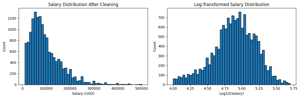
The raw distribution is right-skewed, which is typical for income data. The log-transformed version on the right shows how salaries cluster more naturally in the center when we account for the scale. For linear regression, log-transforming your target variable is worth experimenting with in a next step, since it can help the model perform better on skewed data.
Learning Insight: The \$10k minimum cutoff may be a bit aggressive. Looking at the bottom salary data, some of those \$1/year entries come from countries where cost of living means compensation is often reported differently, or where there may have been a survey misunderstanding. There's room to experiment with different thresholds here. If you want to extend this project, try adjusting the cutoffs and see how the model results change.
Step 4: Engineering Features from Multi-Select Columns
Here's where things get interesting. Several columns in this dataset aren't just single values; they're semicolon-separated lists of everything a developer has worked with. For example, LanguageHaveWorkedWith might look like Python;SQL;JavaScript;TypeScript for a given row.
Machine learning models can't work with strings like that directly, so we need a strategy.
First attempt: count the skills
Our initial hypothesis is that the number of tools someone knows might correlate with their salary.
df_model['Num_Languages'] = df_model['LanguageHaveWorkedWith'].str.count(';') + 1
df_model['Num_Databases'] = df_model['DatabaseHaveWorkedWith'].str.count(';') + 1
df_model['Num_Platforms'] = df_model['PlatformHaveWorkedWith'].str.count(';') + 1
df_model['Num_Webframes'] = df_model['WebframeHaveWorkedWith'].str.count(';') + 1
df_model['Num_Tools'] = df_model['ToolsTechHaveWorkedWith'].str.count(';') + 1

df_model['Total_Skills'] = (
    df_model['Num_Languages'] + df_model['Num_Databases'] +
    df_model['Num_Platforms'] + df_model['Num_Webframes'] + df_model['Num_Tools']
)

print("\nCorrelation with salary:")
count_cols = ['Num_Languages', 'Num_Databases', 'Num_Platforms', 'Num_Webframes', 'Num_Tools', 'Total_Skills']
correlation_data = df_model[count_cols + ['ConvertedCompYearly']].corr()['ConvertedCompYearly'].sort_values(ascending=False)
print(correlation_data)
Correlation with salary:
ConvertedCompYearly 1.000000
Num_Tools 0.114356
Num_Languages 0.074025
Total_Skills 0.044754
Num_Platforms 0.006805
Num_Databases -0.003100
Num_Webframes -0.072698Not great. The number of tools has the highest correlation at just 11%, which is a very weak signal. And by reducing each column to a single count, we lose all the information about which tools someone actually knows. Knowing that someone uses Terraform is much more telling than knowing they use 7 tools.
Better approach: binary features
Instead, we'll explore what the most common individual skills are, then create a binary column for each one indicating whether that developer uses it.
print("Top 20 languages:")
all_langs = df_model['LanguageHaveWorkedWith'].str.split(';').explode()
print(all_langs.value_counts().head(20))

print("\nTop 15 databases:")
all_dbs = df_model['DatabaseHaveWorkedWith'].str.split(';').explode()
print(all_dbs.value_counts().head(15))

print("\nTop 15 platforms:")
all_platforms = df_model['PlatformHaveWorkedWith'].str.split(';').explode()
print(all_platforms.value_counts().head(15))
Top 20 languages:
JavaScript 11851
SQL 9565
HTML/CSS 9423
TypeScript 8868
Python 7193
Bash/Shell (all shells) 6042
C# 5108
Java 4645
PHP 3059
Go 2840
...
Top 15 databases:
PostgreSQL 8827
MySQL 6112
Redis 4865
...
Top 15 platforms:
Amazon Web Services (AWS) 9556
Microsoft Azure 5162
Google Cloud 4082
...Now we can see clearly what the most common tools are. Based on this, we'll create binary (0/1) columns for specific high-value and popular skills across languages, databases, cloud platforms, web frameworks, and DevOps tools.
# Languages: High-paying/specialized
df_model['Has_Rust'] = df_model['LanguageHaveWorkedWith'].str.contains('Rust', na=False).astype(int)
df_model['Has_Go'] = df_model['LanguageHaveWorkedWith'].str.contains('Go', na=False).astype(int)
df_model['Has_Scala'] = df_model['LanguageHaveWorkedWith'].str.contains('Scala', na=False).astype(int)
df_model['Has_Kotlin'] = df_model['LanguageHaveWorkedWith'].str.contains('Kotlin', na=False).astype(int)
df_model['Has_Swift'] = df_model['LanguageHaveWorkedWith'].str.contains('Swift', na=False).astype(int)

# Languages: Popular/versatile
df_model['Has_Python'] = df_model['LanguageHaveWorkedWith'].str.contains('Python', na=False).astype(int)
df_model['Has_JavaScript'] = df_model['LanguageHaveWorkedWith'].str.contains('JavaScript', na=False).astype(int)
df_model['Has_TypeScript'] = df_model['LanguageHaveWorkedWith'].str.contains('TypeScript', na=False).astype(int)
df_model['Has_Java'] = df_model['LanguageHaveWorkedWith'].str.contains('Java', na=False).astype(int)
df_model['Has_CSharp'] = df_model['LanguageHaveWorkedWith'].str.contains('C#', na=False).astype(int)
df_model['Has_SQL'] = df_model['LanguageHaveWorkedWith'].str.contains('SQL', na=False).astype(int)

# Databases
df_model['Has_PostgreSQL'] = df_model['DatabaseHaveWorkedWith'].str.contains('PostgreSQL', na=False).astype(int)
df_model['Has_MongoDB'] = df_model['DatabaseHaveWorkedWith'].str.contains('MongoDB', na=False).astype(int)
df_model['Has_Redis'] = df_model['DatabaseHaveWorkedWith'].str.contains('Redis', na=False).astype(int)
df_model['Has_Elasticsearch'] = df_model['DatabaseHaveWorkedWith'].str.contains('Elasticsearch', na=False).astype(int)

# Cloud platforms
df_model['Has_AWS'] = df_model['PlatformHaveWorkedWith'].str.contains('Amazon Web Services|AWS', na=False).astype(int)
df_model['Has_Azure'] = df_model['PlatformHaveWorkedWith'].str.contains('Azure', na=False).astype(int)
df_model['Has_GCP'] = df_model['PlatformHaveWorkedWith'].str.contains('Google Cloud', na=False).astype(int)

# Web frameworks
df_model['Has_React'] = df_model['WebframeHaveWorkedWith'].str.contains('React', na=False).astype(int)
df_model['Has_NextJS'] = df_model['WebframeHaveWorkedWith'].str.contains('Next.js', na=False).astype(int)
df_model['Has_NodeJS'] = df_model['WebframeHaveWorkedWith'].str.contains('Node.js', na=False).astype(int)
df_model['Has_SpringBoot'] = df_model['WebframeHaveWorkedWith'].str.contains('Spring Boot', na=False).astype(int)

# DevOps/infrastructure tools
df_model['Has_Docker'] = df_model['ToolsTechHaveWorkedWith'].str.contains('Docker', na=False).astype(int)
df_model['Has_Kubernetes'] = df_model['ToolsTechHaveWorkedWith'].str.contains('Kubernetes', na=False).astype(int)
df_model['Has_Terraform'] = df_model['ToolsTechHaveWorkedWith'].str.contains('Terraform', na=False).astype(int)
Now let's check how well these binary features correlate with salary compared to our count approach.
skill_features = [col for col in df_model.columns if col.startswith('Has_')]
skill_corr = df_model[skill_features + ['ConvertedCompYearly']].corr()['ConvertedCompYearly'].sort_values(ascending=False)
print("=== ALL Skill Correlations (sorted) ===")
print(skill_corr[skill_corr.index != 'ConvertedCompYearly'])
=== ALL Skill Correlations (sorted) ===
Has_Terraform 0.177524
Has_AWS 0.142293
Has_Kubernetes 0.128906
Has_Go 0.123166
Has_Rust 0.082603
Has_Python 0.079271
Has_Docker 0.064240
Has_Redis 0.061930
Has_React 0.061303
Has_Elasticsearch 0.053530
Has_PostgreSQL 0.049394
Has_Scala 0.046563
Has_TypeScript 0.037359
Has_GCP 0.035238
Has_Swift 0.023807
Has_Kotlin 0.014656
Has_SQL 0.005919
Has_Azure -0.014817
Has_JavaScript -0.015086
Has_NextJS -0.017373
Has_Java -0.017985
Has_CSharp -0.020396
Has_NodeJS -0.024481
Has_SpringBoot -0.035468
Has_MongoDB -0.095041Terraform, AWS, and Kubernetes are the strongest positive signals, while MongoDB and Spring Boot trend negative. None of these are strong correlations on their own, but together they'll give our model meaningful information to work with.
Learning Insight: It might seem strange that some popular skills like JavaScript and Java have slightly negative correlations with salary. This likely reflects the distribution of who uses them, JavaScript developers include a lot of front-end engineers and early-career learners, while Terraform and Kubernetes users tend to be more senior infrastructure specialists. Correlation doesn't tell the whole story, which is exactly why we're building a model rather than just sorting by correlation values.
Now we drop the original multi-select string columns and our count features, since the binary features replace them.
cols_to_drop_final = [
    'LanguageHaveWorkedWith', 'DatabaseHaveWorkedWith',
    'PlatformHaveWorkedWith', 'WebframeHaveWorkedWith',
    'ToolsTechHaveWorkedWith',
    'Num_Languages', 'Num_Databases', 'Num_Platforms',
    'Num_Webframes', 'Num_Tools', 'Total_Skills'
]
df_model = df_model.drop(columns=cols_to_drop_final)
print(f"Final shape with binary skill features: {df_model.shape}")
print(f"\nFeature types:")
print(df_model.dtypes.value_counts())
Final shape with binary skill features: (15309, 41)
Feature types:
int64 25
object 14
float64 2Good progress. We've got 25 clean integer columns from our binary features, but we still have 14 object columns to deal with. Let's tackle those now.
Step 5: Encoding the Remaining Categorical Columns
Let's get a full picture of what's left.
categorical_cols = df_model.select_dtypes(include='object').columns.tolist()
for col in categorical_cols:
    n_unique = df_model[col].nunique()
    print(f"\n{col}: {n_unique} unique values")
    if n_unique <= 20:
        print(df_model[col].value_counts())
After reviewing the output, here's our encoding plan:
| Column | Unique Values | Strategy |
|---|---|---|
MainBranch |
2 | Boolean (1/0) |
Age |
8 | Ordinal encoding |
EdLevel |
8 | Ordinal encoding |
OrgSize |
10 | Ordinal encoding |
Employment |
10 | Simplify, then one-hot |
RemoteWork |
3 | One-hot encoding |
AISelect |
3 | One-hot encoding |
Industry |
12 | One-hot encoding |
DevType |
33 | Keep top 10, group rest as "Other", one-hot |
Country |
140 | Keep top 15, group rest as "Other", one-hot |
YearsCode |
52 | Coerce to numeric |
YearsCodePro |
51 | Coerce to numeric |
LearnCode |
554 | Drop (too fragmented) |
OpSysProfessional use |
947 | Drop (too fragmented) |
Let's walk through each of these.
Drop the unfixable columns
LearnCode has 554 unique combinations of responses, and OpSysProfessional use has 947. There's no clean way to encode either of these without adding an enormous amount of noise to the model.
df_model = df_model.drop(columns=['LearnCode', 'OpSysProfessional use'])Ordinal encoding for age, education, and organization size
These columns have a natural order to them: a bachelor's degree ranks higher than a high school diploma, and a 10,000-person company ranks larger than a 10-person startup. Ordinal encoding captures that relationship by assigning a number to each category.
age_order = {
    'Under 18 years old': 0, '18-24 years old': 1,
    '25-34 years old': 2, '35-44 years old': 3,
    '45-54 years old': 4, '55-64 years old': 5,
    '65 years or older': 6, 'Prefer not to say': 2
}
df_model['Age_Ordinal'] = df_model['Age'].map(age_order)
df_model = df_model.drop(columns=['Age'])

edlevel_order = {
    'Primary/elementary school': 0,
    'Secondary school (e.g. American high school, German Realschule or Gymnasium, etc.)': 1,
    'Some college/university study without earning a degree': 2,
    'Associate degree (A.A., A.S., etc.)': 3,
    "Bachelor's degree (B.A., B.S., B.Eng., etc.)": 4,
    "Master's degree (M.A., M.S., M.Eng., MBA, etc.)": 5,
    'Professional degree (JD, MD, Ph.D, Ed.D, etc.)': 6,
    'Something else': 2
}
df_model['EdLevel_Ordinal'] = df_model['EdLevel'].map(edlevel_order)
df_model = df_model.drop(columns=['EdLevel'])

orgsize_order = {
    'Just me - I am a freelancer, sole proprietor, etc.': 0,
    '2 to 9 employees': 1, '10 to 19 employees': 2,
    '20 to 99 employees': 3, '100 to 499 employees': 4,
    '500 to 999 employees': 5, '1,000 to 4,999 employees': 6,
    '5,000 to 9,999 employees': 7, '10,000 or more employees': 8,
    "I don't know": 4
}
df_model['OrgSize_Ordinal'] = df_model['OrgSize'].map(orgsize_order)
df_model = df_model.drop(columns=['OrgSize'])
Simplifying employment status
Employment has 10 unique combinations, many of them overlapping. We simplify these down to four categories based on what matters most.
def simplify_employment(emp):
    if pd.isna(emp):
        return 'Unknown'
    elif 'Employed, full-time' in emp and 'Independent contractor' in emp:
        return 'Full-time + Freelance'
    elif 'Employed, full-time' in emp:
        return 'Full-time'
    elif 'Independent contractor' in emp or 'freelancer' in emp or 'self-employed' in emp:
        return 'Freelance'
    elif 'part-time' in emp:
        return 'Part-time'
    else:
        return 'Other'

df_model['Employment_Simple'] = df_model['Employment'].apply(simplify_employment)
df_model = df_model.drop(columns=['Employment'])

print("\nSimplified Employment:")
print(df_model['Employment_Simple'].value_counts())
Simplified Employment:
Employment_Simple
Full-time 12776
Full-time + Freelance 1462
Freelance 866
Part-time 205One-hot encoding low-cardinality columns
For columns with a small number of unique values and no natural ordering, we use pd.get_dummies(). This creates a new binary column for each category, so a column like RemoteWork with values of Remote, Hybrid, and In-person becomes three separate 0/1 columns.
one_hot_cols = ['MainBranch', 'RemoteWork', 'AISelect', 'Employment_Simple']
for col in one_hot_cols:
    dummies = pd.get_dummies(df_model[col], prefix=col, drop_first=True)
    df_model = pd.concat([df_model, dummies], axis=1)
    df_model = df_model.drop(columns=[col])

industry_dummies = pd.get_dummies(df_model['Industry'], prefix='Industry', drop_first=True)
df_model = pd.concat([df_model, industry_dummies], axis=1)
df_model = df_model.drop(columns=['Industry'])
Coercing years of experience to numeric
YearsCode and YearsCodePro should be numbers, but they're stored as objects because some responses include text like "Less than 1 year". We convert them to numeric and let anything non-numeric become a null, which we'll clean up shortly.
df_model['YearsCode'] = pd.to_numeric(df_model['YearsCode'], errors='coerce')
df_model['YearsCodePro'] = pd.to_numeric(df_model['YearsCodePro'], errors='coerce')
Handling high-cardinality columns: DevType and Country
DevType has 33 unique values and Country has 140. One-hot encoding these directly would add a huge number of columns, most of which would have very little data. Instead, we keep the most common values and group everything else into "Other".
# DevType: keep top 10
top_10_devtypes = df_model['DevType'].value_counts().head(10).index
df_model['DevType_Grouped'] = df_model['DevType'].apply(
    lambda x: x if x in top_10_devtypes else 'Other'
)
devtype_dummies = pd.get_dummies(df_model['DevType_Grouped'], prefix='DevType', drop_first=True)
df_model = pd.concat([df_model, devtype_dummies], axis=1)
df_model = df_model.drop(columns=['DevType', 'DevType_Grouped'])

# Country: keep top 15
top_15_countries = df_model['Country'].value_counts().head(15).index
df_model['Country_Grouped'] = df_model['Country'].apply(
    lambda x: x if x in top_15_countries else 'Other'
)
country_dummies = pd.get_dummies(df_model['Country_Grouped'], prefix='Country', drop_first=True)
df_model = pd.concat([df_model, country_dummies], axis=1)
df_model = df_model.drop(columns=['Country', 'Country_Grouped'])
Let's verify our work.
print(f"\nColumn types:")
print(df_model.dtypes.value_counts())
print(f"\nAll numeric? {df_model.select_dtypes(include='object').shape[1] == 0}")

null_counts = df_model.isnull().sum()
print(f"\nRemaining nulls:")
print(null_counts[null_counts > 0])
Column types:
bool 44
int64 27
float64 5
All numeric? True
Remaining nulls:
YearsCode 20
YearsCodePro 236
OrgSize_Ordinal 140No more object columns. We introduced a small number of nulls during the numeric coercion step, so we'll do one final drop.
df_model = df_model.dropna()
print(f"\nShape after dropping nulls: {df_model.shape}")
print(f"Rows lost: {15309 - len(df_model)}")
print(f"Percentage retained: {len(df_model)/15309*100:.1f}%")

print(f"\n=== FINAL CLEAN DATASET ===")
print(f"Rows: {len(df_model)}")
print(f"Columns: {df_model.shape[1]}")
print(f"Features: {df_model.shape[1] - 1}")
print(f"Target: ConvertedCompYearly")
Shape after dropping nulls: (14924, 76)
Rows lost: 385
Percentage retained: 97.5%
=== FINAL CLEAN DATASET ===
Rows: 14924
Columns: 76
Features: 75
Target: ConvertedCompYearlyWe retained 97.5% of our data in this final step. We now have a clean, fully numeric dataset with 14,924 rows and 75 features, ready for modeling.
Learning Insight: We went from 33 columns to 76 columns. That might seem like a lot, but most of those new columns came from one-hot encoding categorical variables. Each binary column is just a yes/no signal, and a well-structured linear model can handle this number of features well. In Part 2, we'll also trim the features that contribute very little signal before training.
What We Built
Let's recap the transformation pipeline we just built:
- Dropped 12 columns with >50% missing data or low relevance to salary
- Removed rows with any remaining null values, bringing us from 48,019 to 16,460 rows
- Filtered salary outliers below \$10,000 and above \$500,000
- Explored count-based features for multi-select skill columns, then replaced them with 25 binary skill indicators
- Applied ordinal encoding to
Age,EdLevel, andOrgSize - Simplified and one-hot encoded
Employment,RemoteWork,AISelect, andIndustry - Grouped high-cardinality columns (
DevType,Country) and one-hot encoded the results - Coerced years experience columns to numeric and dropped the remaining nulls
That's a substantial pipeline, and every step required judgment calls about tradeoffs between keeping data and maintaining quality. The decisions we made here will directly affect how the model performs in Part 2.
Next Steps
In Part 2, we'll take this clean dataset and build the actual salary prediction model. We'll calculate feature correlations with salary, address multicollinearity among the experience columns, train a linear regression model, and then interpret what the results tell us about what actually drives developer compensation.
In the meantime, head into the Dataquest app to work through the project yourself. The solution notebook is available for reference on GitHub. If you hit any snags, drop a question in the Dataquest Community Forum.
If you're newer to machine learning concepts and want to build a stronger foundation before diving in, check out the Machine Learning in Python course. It covers the core ideas behind supervised learning, linear regression, and model evaluation that we'll be applying in Part 2.
from Dataquest https://ift.tt/ufMUFEv
via RiYo Analytics


No comments