Sequence Models in PyTorch

https://ift.tt/fa5W3DM As data scientists, we often work with data where each observation is treated as independent from others. Traditiona...

https://ift.tt/fa5W3DM

As data scientists, we often work with data where each observation is treated as independent from others. Traditional machine learning models like linear regression or random forests make this same assumption ― they see each data point as a standalone entity with no relationship to what came before or after. This approach works well for many problems but falls apart when dealing with data where order matters.

Think about predicting tomorrow's stock price or guessing the next word in a sentence. Each data point connects to what came before it. Today's stock price shapes tomorrow's movement. The first few words in a sentence limit what words can logically follow. These sequential relationships contain valuable insights that traditional machine learning models simply can't capture.

Introducing Sequence Models

Luckily, these sequential relationships can be modeled using a type of neural network called sequence models that can track patterns over time. In a moment, we’ll get our hands dirty by exploring three different types of sequence models. Each one builds on the previous, helping us understand how neural networks can learn from time-based patterns.

You'll need some PyTorch basics like tensors, simple models, and training loops to follow along. If you need a refresher, check out our Getting Started with PyTorch tutorial first.

Why Sequence Models Matter for Data Scientists

Many data problems involve more than just a snapshot in time; they often involve change, progression, and patterns that unfold. Sequence models are designed to capture exactly that. Sequence models power many tools data scientists use daily:

• Business forecasting helps companies predict sales trends, inventory needs, and resource demands. Businesses use these predictions to make smarter decisions about staffing, purchases, and production schedules.
• Financial prediction enables spotting market trends before others. Analysts use these insights for smarter trading, better risk management, and detecting market anomalies.
• Customer analysis reveals patterns in purchasing behavior over time. Companies use this to improve recommendations, personalize marketing, and predict which customers might leave.
• Anomaly detection identifies unusual patterns in streaming data. Manufacturers use this to spot equipment problems before failures happen, saving on maintenance costs and preventing downtime.

As a data scientist, you’ll encounter projects where the when is just as important as the what. Sequence models let you move beyond static patterns and capture how things evolve — something classical models simply can't do. Understanding how to apply them expands the kinds of problems you can solve, the insights you can uncover, and the value you can deliver.

Benefits Over Traditional Methods

Compared to simpler approaches like linear regression or basic machine learning models applied to time series, sequence models offer several advantages:

• They automatically learn patterns over time without requiring manual feature engineering
• They can capture complex relationships that simpler models miss
• They adapt to changing trends in your data
• They handle multiple input variables naturally

Our Cinema Ticket Sales Case Study

Throughout this tutorial, we'll focus on forecasting cinema ticket sales by building and training sequential models that learn from patterns in prior sales. This example works well because:

1. It has clear time patterns (weekend spikes, seasonality)
2. It represents a real business need with tangible impacts
3. The results are easy to visualize and understand

By predicting future ticket sales, cinema owners can make smarter decisions about staffing, inventory, and promotions. Good forecasts mean better profits and fewer wasted resources.

Understanding Sequence Models

Now let's see how these models work and why they're perfect for our ticket sales forecast.

Why Standard Networks Aren't Enough for Our Ticket Sales

Imagine trying to predict Saturday's ticket sales with a standard neural network. You might input features like "day of week" or "month." The model would try to map these directly to expected sales.

But this misses crucial patterns. Is there an upward trend? Did sales drop last weekend? Standard neural networks can't "remember" this context.

The problem? Feed-forward networks have no memory. They process each input independently, with no knowledge of what came before.

A feed-forward network (left) processes each input independently, while an RNN (right) maintains "memory" of previous inputs through recurrent connections.

Recurrent Neural Networks: Adding Memory

Recurrent Neural Networks (RNNs) solve this with a simple but powerful idea: recurrent connections. Besides sending outputs forward, RNNs pass information sideways through time, creating memory.

This memory allows the network to:

• Find patterns that develop over time
• Carry information from earlier steps to later ones
• Learn how sequence elements depend on each other

For our cinema ticket sales, this means the model can learn that Friday sales often predict Saturday sales, or recognize seasonal patterns around blockbuster releases.

PyTorch's RNN Building Blocks

PyTorch makes building RNNs straightforward with the torch.nn module. The main options include:

• nn.RNN: Basic recurrent neural network
• nn.LSTM: Long Short-Term Memory (better for longer sequences)
• nn.GRU: Gated Recurrent Unit (efficient alternative to LSTM)

We'll explore each one, starting with the simplest approach.

Preparing Time Series Data for PyTorch

Before building any of these sequential models, we need to prepare our data. Good preparation makes or breaks sequence models. Let’s explore the data to learn how to best prepare it for training.

Our Cinema Ticket Sales Dataset

Our dataset contains daily ticket sales from a cinema over several months. Let's load it and take a look at its line plot:

import pandas as pd
import numpy as np
import matplotlib.pyplot as plt
import torch

sales_data = pd.read_csv("cinema_data.csv", 
                          parse_dates=['date'], 
                          index_col='date'
)

print(sales_data.head())

plt.figure(figsize=(12, 6))
plt.plot(sales_data['total_sales'])
plt.title('Daily Cinema Ticket Sales')
plt.xlabel('Date')
plt.ylabel('Total Sales')
plt.grid(True)
plt.show()

            total_sales
date                   
2018-03-14     63720000
2018-03-15    195080000
2018-03-16    204720000
2018-03-17     59980000
2018-03-18     74720000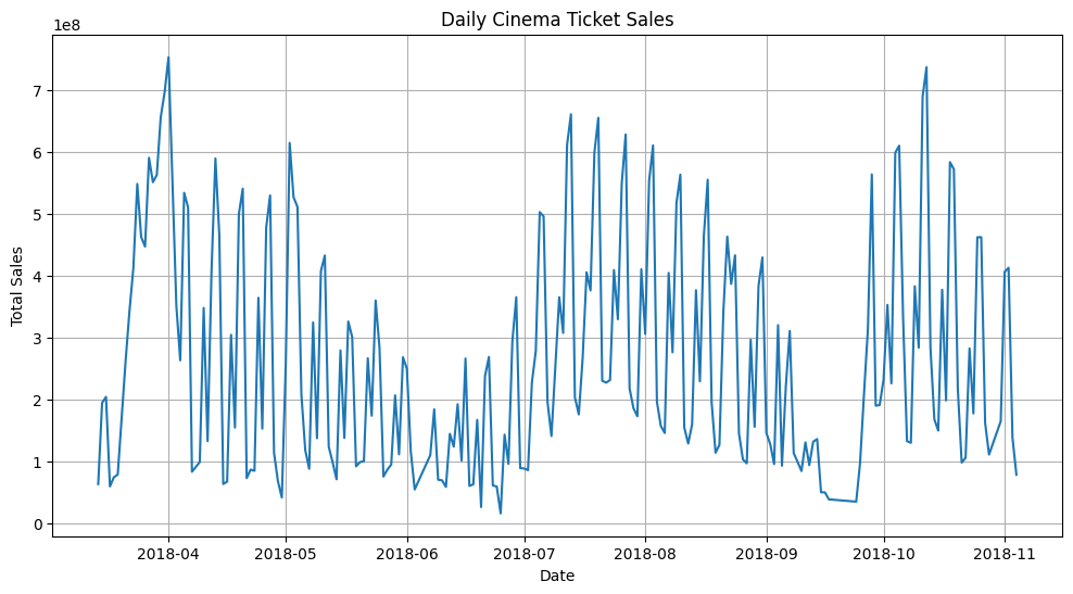

Looking at the plot, we can see:

• Weekend spikes in ticket sales
• Occasional larger spikes (likely blockbuster releases)
• Some seasonal trends

Creating Time Windows for Sequence Prediction

Before we can train a sequence model, we need to reshape our data into "windows" — sequences of consecutive days that the model can learn from. Each window contains a set of previous values the model will use to predict the next one.

Because cinema ticket sales tend to follow weekly patterns, we'll use sequences that span at least one full week. This gives the model a better chance to learn those recurring rhythms. We'll create a simple function to handle this preprocessing step for us:

def create_sequence_data(data, window_size=1):
    """
    Create sequences of data for time series forecasting.

    Args:
        data: DataFrame with time series data
        window_size: Number of previous time steps to use

    Returns:
        X: Input sequences [samples, window_size, features]
        y: Target values [samples, 1]
    """
    X, y = [], []

    # Convert DataFrame to NumPy array if needed
    if isinstance(data, pd.DataFrame):
        data_array = data.values
    else:
        data_array = data

    # Create sequences
    for i in range(len(data_array) - window_size):
        # Get window_size time steps for input X
        window = data_array[i:(i + window_size)]
        # Get the next value as target y
        target = data_array[i + window_size]

        X.append(window)
        y.append(target)

    return np.array(X), np.array(y)

# Create sequences with 9 days as input to predict the 10th day
window_size = 9  
X, y = create_sequence_data(sales_data[['total_sales']], window_size)

print(f"X shape: {X.shape}")
print(f"y shape: {y.shape}")
print(f"Example sequence: {X[0].flatten()}")
print(f"Example target: {y[0][0]}")

X shape: (213, 9, 1)
y shape: (213, 1)
Example sequence: [ 63720000  195080000  204720000  59980000  74720000  79140000  261750000  342900000  412950000 ]
Example target: 548900000

The X array now contains sequences of 9 days of sales, and the y array contains the sales for the following day.

Splitting into Training and Testing Sets

Next, we split our data into training and testing sets:

from sklearn.model_selection import train_test_split

# Split the data (without shuffling to maintain time order)
X_train, X_test, y_train, y_test = train_test_split(
    X, y, test_size=0.15, shuffle=False
)

print(f"Training data: {X_train.shape}")
print(f"Testing data:  {X_test.shape}")

Training data: (181, 9, 1)
Testing data:  (32, 9, 1)

Notice we set shuffle=False. For time series data, we must maintain the temporal order.

Setting a Seed and Scaling the Data

Building neural networks always involves some level of randomness — especially during the initial weight assignment in model layers. Setting a seed value ensures reproducibility by keeping that randomness consistent across code runs.

Neural networks also tend to perform better when inputs are on a consistent scale. To help our models train more effectively, we'll normalize our data by scaling the training data to fall within a 0–1 range.

import random
from sklearn.preprocessing import MinMaxScaler

# Set seed values for reproducibility
SEED = 42
random.seed(SEED)
np.random.seed(SEED)
torch.manual_seed(SEED)

# Fit scaler on training data only
scaler = MinMaxScaler()
X_train_scaled = scaler.fit_transform(X_train.reshape(-1, 1)).reshape(X_train.shape)

# Apply that same scaler to target and test data as well
y_train_scaled = scaler.transform(y_train.reshape(-1, 1))
X_test_scaled = scaler.transform(X_test.reshape(-1, 1)).reshape(X_test.shape)
y_test_scaled = scaler.transform(y_test.reshape(-1, 1))

print(f"X_train_scaled range: [{X_train_scaled.min():.4f}, {X_train_scaled.max():.4f}]")
print(f"y_train_scaled range: [{y_train_scaled.min():.4f}, {y_train_scaled.max():.4f}]")
print(f"X_test_scaled range:  [{X_test_scaled.min():.4f}, {X_test_scaled.max():.4f}]")
print(f"y_test_scaled range:  [{y_test_scaled.min():.4f}, {y_test_scaled.max():.4f}]")

X_train_scaled range: [0.0000, 1.0000]
y_train_scaled range: [0.0000, 1.0000]
X_test_scaled range:  [0.0256, 0.9781]
y_test_scaled range:  [0.0847, 0.9781]

Did you notice we scaled the data after splitting it into training and test sets? This is an easy detail to miss, but it protects us from a common mistake: data leakage.

Data leakage happens when information from outside the training set — like the distribution of the test set — influences the model during training. It often goes unnoticed but can lead to overly optimistic results and poor generalization.

By calling fit_transform() only on the training data, and transform() on the test data, we ensure that scaling parameters come only from data the model is allowed to see. This keeps our evaluation honest and prevents subtle contamination between training and test sets.

It’s a small detail, but one that separates reliable models from misleading ones. Many data scientists overlook it. Now you won’t.

Converting to PyTorch Tensors

Finally, we convert our NumPy arrays to PyTorch tensors:

X_train_tensor = torch.tensor(X_train_scaled, dtype=torch.float32)
y_train_tensor = torch.tensor(y_train_scaled, dtype=torch.float32)
X_test_tensor = torch.tensor(X_test_scaled, dtype=torch.float32)
y_test_tensor = torch.tensor(y_test_scaled, dtype=torch.float32)

print(f"X_train_tensor shape: {X_train_tensor.shape}")
print(f"y_train_tensor shape: {y_train_tensor.shape}")
print(f"X_test_tensor shape:  {X_test_tensor.shape}")
print(f"y_test_tensor shape:  {y_test_tensor.shape}")

X_train_tensor shape: torch.Size([181, 9, 1])
y_train_tensor shape: torch.Size([181, 1])
X_test_tensor shape:  torch.Size([32, 9, 1])
y_test_tensor shape:  torch.Size([32, 1])

There, our data is ready for modeling! We have:

• Sequences of 9 days of sales as inputs
• The next day's sales as targets
• All values scaled to the 0-1 range, based on the training data
• Everything converted to PyTorch tensors

Building a Simple RNN Model for Ticket Sales

Let's start with a basic RNN model for our cinema ticket sales forecast.

Basic RNN Implementation

Before jumping into the model architecture, we’ll first define a few common parameters that control how the model learns — things like the number of neurons in each layer, how many sequences the model sees at a time, and how fast it updates during training. These choices have a big impact on performance, and one of the best ways to build intuition is to experiment with them. Try tweaking values like the number of epochs, hidden layer sizes, or learning rate to see how your results change.

import torch.nn as nn

# Define model parameters for all models
num_rec_layers = 1       # Number of recurrent layers in the model
rec_hidden_size = 32     # Neurons in hidden recurrent layer
fc_hidden1_size = 16     # Neurons in first fully connected hidden layer
fc_hidden2_size = 8      # Neurons in second fully connected hidden layer
output_size = 1          # Predicting a single value
batch_size = 32          # Sequences per batch
num_epochs = 100         # Training iterations
learning_rate = 0.01    # Learning rate for optimizer

# Recurrent neural network (RNN) layer
rnn_layer = nn.RNN(
    input_size=1,
    hidden_size=rec_hidden_size,
    num_layers=num_rec_layers,
    batch_first=True
)

# Intermediate fully-connected hidden layers
fc_hidden1 = nn.Linear(rec_hidden_size, fc_hidden1_size)
fc_hidden2 = nn.Linear(fc_hidden1_size, fc_hidden2_size)

# Fully-connected output layer
fc_output = nn.Linear(fc_hidden2_size, output_size)

# Loss function and optimizer
loss_fn = nn.MSELoss()
optimizer = torch.optim.Adam([
    {'params': rnn_layer.parameters()},
    {'params': fc_hidden1.parameters()},
    {'params': fc_hidden2.parameters()},
    {'params': fc_output.parameters()}
], lr=learning_rate)

# Initialize hidden state for recurrent layer
# The hidden state acts as the model’s short-term memory.
# Before the sequence starts, we initialize it to all zeros —
# a clean slate for the model to begin learning from.
def init_rnn_hidden(batch_size):
    return torch.zeros(num_rec_layers, batch_size, rec_hidden_size)

# Display model structure
print("RNN layer:                          ", rnn_layer)
print("First fully-connected hidden layer: ", fc_hidden1)
print("Second fully-connected hidden layer:", fc_hidden2)
print("Fully-connected output layer:       ", fc_output)

RNN layer:                           RNN(1, 32, batch_first=True)
First fully-connected hidden layer:  Linear(in_features=32, out_features=16, bias=True)
Second fully-connected hidden layer: Linear(in_features=16, out_features=8, bias=True)
Fully-connected output layer:        Linear(in_features=8, out_features=1, bias=True)

Training the RNN Model

Now let's train our model:

import torch.nn.functional as F

# List to store training losses per epoch
rnn_train_losses = []

# Training loop
for epoch in range(num_epochs):
    # Track total loss and batch count for averaging
    epoch_loss = 0.0
    num_batches = 0

    # Process training data in batches
    for i in range(0, len(X_train_tensor), batch_size):
        # Select the current batch of sequences
        batch_X = X_train_tensor[i:i+batch_size]
        batch_y = y_train_tensor[i:i+batch_size]

        # Handle last batch size adjustment if needed
        current_batch_size = batch_X.shape[0]

        # Initialize hidden state for the current batch
        h_0 = init_rnn_hidden(current_batch_size)

        # Forward pass
        # Step 1: Pass sequences through the recurrent layer
        rnn_out, _ = rnn_layer(batch_X, h_0)

        # Step 2: Extract output from the last timestep
        last_output = rnn_out[:, -1, :]

        # Step 3: Pass through fully-connected layers with ReLU activation
        hidden_out1 = F.relu(fc_hidden1(last_output))
        hidden_out2 = F.relu(fc_hidden2(hidden_out1))

        # Step 4: Pass through final output layer to generate predictions
        predictions = fc_output(hidden_out2)

        # Compute loss between predictions and actual values
        loss = loss_fn(predictions, batch_y)

        # Backpropagation and parameter updates
        optimizer.zero_grad()   # Clear gradients
        loss.backward()         # Compute gradients
        optimizer.step()        # Update parameters

        # Accumulate loss for averaging
        epoch_loss += loss.item()
        num_batches += 1

    # Compute average loss for the epoch
    avg_loss = epoch_loss / num_batches
    rnn_train_losses.append(avg_loss)

    # Print training progress every 10 epochs
    if (epoch + 1) % 10 == 0:
        print(f'Epoch [{epoch+1}/{num_epochs}], Loss: {avg_loss:.4f}')

# Plot training loss curve
plt.figure(figsize=(10, 5))
plt.plot(rnn_train_losses)
plt.title('RNN Training Loss')
plt.xlabel('Epoch')
plt.ylabel('Loss')
plt.grid(True)
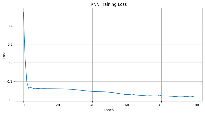
plt.show()

Epoch [10/100], Loss: 0.0601
Epoch [20/100], Loss: 0.0589
Epoch [30/100], Loss: 0.0549
Epoch [40/100], Loss: 0.0455
Epoch [50/100], Loss: 0.0411
Epoch [60/100], Loss: 0.0274
Epoch [70/100], Loss: 0.0220
Epoch [80/100], Loss: 0.0247
Epoch [90/100], Loss: 0.0166
Epoch [100/100], Loss: 0.0158

As training progresses, we can see the loss steadily decreasing across epochs — a sign that the model is learning to minimize its prediction error. While loss values alone don’t tell the full story, they give us a useful early indication that the model is improving during training.

Evaluating the RNN Model

Let's evaluate our model on the test data:

from sklearn.metrics import r2_score

# Set layers to evaluation mode
rnn_layer.eval()
fc_hidden1.eval()
fc_hidden2.eval()
fc_output.eval()

# No gradient computation required for evaluation
with torch.no_grad():
    # Initialize hidden state for test data
    h_0 = init_rnn_hidden(len(X_test_tensor))

    # Forward pass
    rnn_out, _ = rnn_layer(X_test_tensor, h_0)
    last_output = rnn_out[:, -1, :]
    hidden_out1 = F.relu(fc_hidden1(last_output))       
    hidden_out2 = F.relu(fc_hidden2(hidden_out1))

    # Generate predictions
    predictions = fc_output(hidden_out2)                 

    # Convert actual values back to original scale
    y_test_np = y_test_tensor.numpy()
    y_test_original = scaler.inverse_transform(y_test_np)

    # Convert predictions back to original scale
    predictions_np = predictions.numpy()
    predictions_original = scaler.inverse_transform(predictions_np)

    # Calculate and display R² Score
    rnn_r2 = r2_score(y_test_original, predictions_original)
    print(f"RNN R² Score: {rnn_r2:.2f}")

# Visualize actual vs predicted sales
plt.figure(figsize=(12, 6))
plt.plot(y_test_original, label='Actual Sales')
plt.plot(predictions_original, label='Predicted Sales', alpha=0.7)
plt.title('Cinema Ticket Sales: Actual vs Predicted (RNN)')
plt.xlabel('Day')
plt.ylabel('Total Sales')
plt.legend()
plt.grid(True)
plt.show()

RNN R² Score: 0.51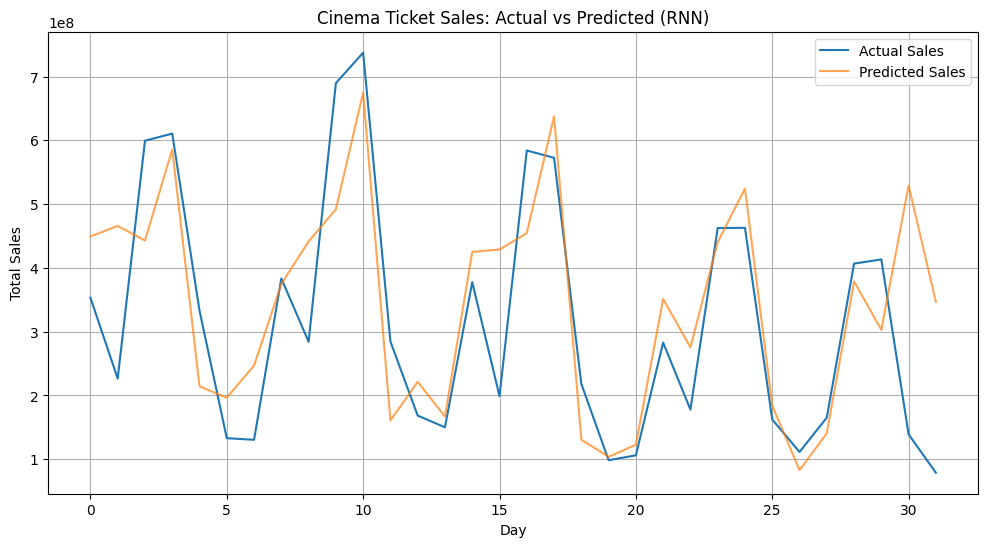

Our simple RNN model captures some patterns in the ticket sales, but struggles with longer-term dependencies. Simple RNNs often have trouble maintaining information over many time steps.

Next, let's try another model type to address this limitation.

Using LSTM for Better Forecasting

Basic RNNs struggle with longer sequences because of the vanishing gradient problem. As information flows through many time steps, the gradients can become too small to be useful.

Long Short-Term Memory (LSTM) networks solve this problem. They use special gates to control what information to remember or forget:

The LSTM cell has gates that control information flow, allowing it to maintain important information over many time steps.

Building an LSTM Model

Let's implement an LSTM model to see how much better its predictions are over our RNN model:

lstm_layer = nn.LSTM(
    input_size=1,
    hidden_size=rec_hidden_size,
    num_layers=1,
    batch_first=True
)
fc_hidden1 = nn.Linear(rec_hidden_size, fc_hidden1_size)
fc_hidden2 = nn.Linear(fc_hidden1_size, fc_hidden2_size)
fc_output = nn.Linear(fc_hidden2_size, output_size)
loss_fn = nn.MSELoss()
optimizer = torch.optim.Adam([
    {'params': lstm_layer.parameters()},
    {'params': fc_hidden1.parameters()},
    {'params': fc_hidden2.parameters()},
    {'params': fc_output.parameters()}
], lr=learning_rate)

# LSTMs track both short (h) and long-term (c) memory
def init_lstm_hidden(batch_size):
    return (torch.zeros(num_rec_layers, batch_size, rec_hidden_size),  # (h)
            torch.zeros(num_rec_layers, batch_size, rec_hidden_size))  # (c)            
print("LSTM layer:                         ", lstm_layer)
print("First fully-connected hidden layer: ", fc_hidden1)
print("Second fully-connected hidden layer:", fc_hidden2)
print("Fully-connected output layer:       ", fc_output)

LSTM layer:                          LSTM(1, 32, batch_first=True)
First fully-connected hidden layer:  Linear(in_features=32, out_features=16, bias=True)
Second fully-connected hidden layer: Linear(in_features=16, out_features=8, bias=True)
Fully-connected output layer:        Linear(in_features=8, out_features=1, bias=True)

Training the LSTM Model

Now let's train our LSTM model:

lstm_train_losses = []

for epoch in range(num_epochs):
    epoch_loss = 0.0
    num_batches = 0
    for i in range(0, len(X_train_tensor), batch_size):
        batch_X = X_train_tensor[i:i+batch_size]
        batch_y = y_train_tensor[i:i+batch_size]
        current_batch_size = batch_X.shape[0]
        h_0, c_0 = init_lstm_hidden(current_batch_size)
        lstm_out, (h_n, c_n) = lstm_layer(batch_X, (h_0, c_0))
        last_output = lstm_out[:, -1, :]
        hidden_out1 = F.relu(fc_hidden1(last_output))
        hidden_out2 = F.relu(fc_hidden2(hidden_out1))
        predictions = fc_output(hidden_out2)
        loss = loss_fn(predictions, batch_y)
        optimizer.zero_grad()
        loss.backward()
        optimizer.step()
        epoch_loss += loss.item()
        num_batches += 1

    avg_loss = epoch_loss / num_batches
    lstm_train_losses.append(avg_loss)

    if (epoch + 1) % 10 == 0:
        print(f'Epoch [{epoch+1}/{num_epochs}], Loss: {avg_loss:.4f}')

plt.figure(figsize=(10, 5))
plt.plot(lstm_train_losses)
plt.title('LSTM Training Loss')
plt.xlabel('Epoch')
plt.ylabel('Loss')
plt.grid(True)
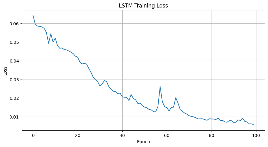
plt.show()

Epoch [10/100], Loss: 0.0499
Epoch [20/100], Loss: 0.0424
Epoch [30/100], Loss: 0.0288
Epoch [40/100], Loss: 0.0227
Epoch [50/100], Loss: 0.0159
Epoch [60/100], Loss: 0.0154
Epoch [70/100], Loss: 0.0113
Epoch [80/100], Loss: 0.0089
Epoch [90/100], Loss: 0.0078
Epoch [100/100], Loss: 0.0056

Compared to the RNN, our LSTM model shows a more rapid and consistent drop in training loss — a sign that its gated architecture is helping it learn more effectively from the data. As before, loss isn’t the full story, but this trend is a promising signal that the LSTM may generalize better during evaluation.

Evaluating the LSTM Model

Let's evaluate our LSTM model and compare it with the simple RNN:

lstm_layer.eval()
fc_hidden1.eval()
fc_hidden2.eval()
fc_output.eval()

with torch.no_grad():
    h_0, c_0 = init_lstm_hidden(len(X_test_tensor))
    lstm_out, _ = lstm_layer(X_test_tensor, (h_0, c_0))
    last_output = lstm_out[:, -1, :]
    hidden_out1 = F.relu(fc_hidden1(last_output))
    hidden_out2 = F.relu(fc_hidden2(hidden_out1))
    predictions = fc_output(hidden_out2)
    predictions_np = predictions.numpy()
    predictions_original = scaler.inverse_transform(predictions_np)
    lstm_r2 = r2_score(y_test_original, predictions_original)

    print("\nModel Comparison:")
    print(f"RNN R²: {rnn_r2:.2f}")
    print(f"LSTM R²: {lstm_r2:.2f}")

plt.figure(figsize=(12, 6))
plt.plot(y_test_original, label='Actual Sales')
plt.plot(predictions_original, label='LSTM Predictions', alpha=0.7)
plt.title('Cinema Ticket Sales: Actual vs Predicted (LSTM)')
plt.xlabel('Day')
plt.ylabel('Total Sales')
plt.legend()
plt.grid(True)
plt.show()

Model Comparison:
RNN R²: 0.51
LSTM R²: 0.58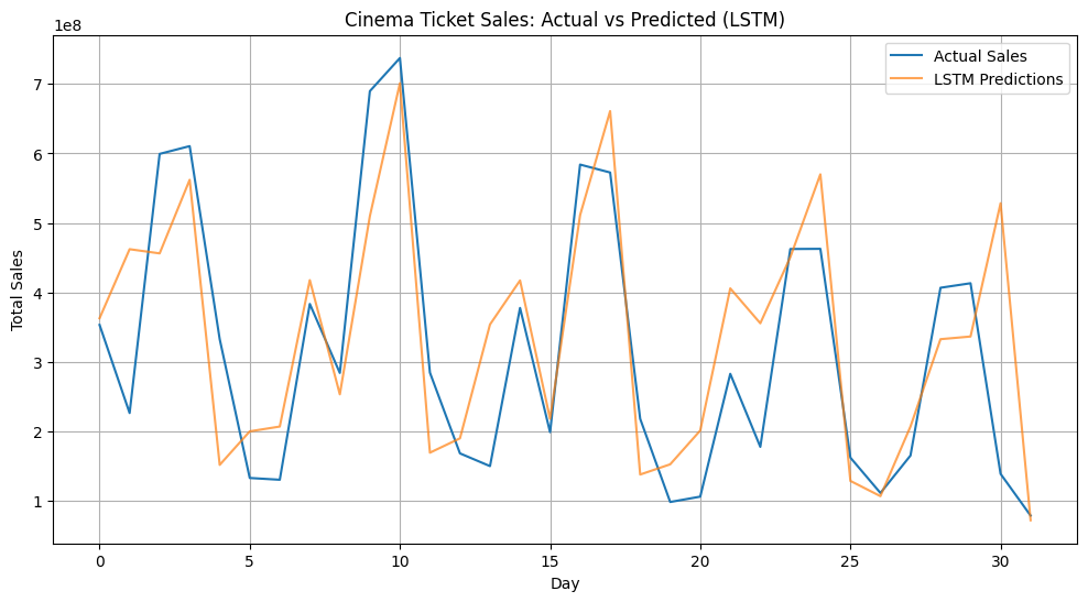

Compared to the RNN model, the LSTM model produces noticeably tighter predictions — particularly in areas with rapid spikes or weekly fluctuations. You might notice improvements such as:

• Stronger alignment with sharp peaks and drops, especially around high-variance regions
• More consistent tracking of week-to-week trends, where the RNN tended to lag or overcorrect
• Reduced noise in low-activity periods, showing better stability across quieter stretches

These gains reflect the LSTM’s strength in capturing temporal dependencies. Its internal memory structure allows it to retain and use patterns from previous time steps more effectively than a basic RNN.

To wrap things up, we’ll test one final model architecture: the Gated Recurrent Unit (GRU). GRUs offer many of the benefits of LSTMs, but with a simpler structure — making them an interesting middle ground between complexity and performance.

Using GRU for Efficient Sequence Modeling

A popular alternative to LSTMs, GRUs are designed to capture long-term dependencies like LSTMs but use a simpler structure with fewer gates. This often makes them faster to train while still retaining strong performance in many sequence modeling tasks.

Below is a diagram of the GRU architecture, which highlights its key components.

GRUs combine the forget and input gates into a single "update gate," making them more efficient.

Let's implement a GRU model using a similar architecture to our previous two models:

gru_layer = nn.GRU(
    input_size=1,
    hidden_size=rec_hidden_size,
    num_layers=1,
    batch_first=True
)
fc_hidden1 = nn.Linear(rec_hidden_size, fc_hidden1_size)
fc_hidden2 = nn.Linear(fc_hidden1_size, fc_hidden2_size)
fc_output = nn.Linear(fc_hidden2_size, output_size)
loss_fn = nn.MSELoss()
optimizer = torch.optim.Adam([
    {'params': gru_layer.parameters()},
    {'params': fc_hidden1.parameters()},
    {'params': fc_hidden2.parameters()},
    {'params': fc_output.parameters()}
], lr=learning_rate)

def init_gru_hidden(batch_size):
    return torch.zeros(num_rec_layers, batch_size, rec_hidden_size)

print("GRU layer:                          ", gru_layer)
print("First fully-connected hidden layer: ", fc_hidden1)
print("Second fully-connected hidden layer:", fc_hidden2)
print("Fully-connected output layer:       ", fc_output)

GRU layer:                           GRU(1, 32, batch_first=True)
First fully-connected hidden layer:  Linear(in_features=32, out_features=16, bias=True)
Second fully-connected hidden layer: Linear(in_features=16, out_features=8, bias=True)
Fully-connected output layer:        Linear(in_features=8, out_features=1, bias=True)

Training and Evaluating the GRU Model

Let's train our GRU model:

gru_train_losses = []

for epoch in range(num_epochs):
    epoch_loss = 0.0
    num_batches = 0
    for i in range(0, len(X_train_tensor), batch_size):
        batch_X = X_train_tensor[i:i+batch_size]
        batch_y = y_train_tensor[i:i+batch_size]
        current_batch_size = batch_X.shape[0]
        h_0 = init_gru_hidden(current_batch_size)
        gru_out, _ = gru_layer(batch_X, h_0)
        last_output = gru_out[:, -1, :]
        hidden_out1 = F.relu(fc_hidden1(last_output))
        hidden_out2 = F.relu(fc_hidden2(hidden_out1))
        predictions = fc_output(hidden_out2)
        loss = loss_fn(predictions, batch_y)
        optimizer.zero_grad()
        loss.backward()
        optimizer.step()
        epoch_loss += loss.item()
        num_batches += 1

    avg_loss = epoch_loss / num_batches
    gru_train_losses.append(avg_loss)

    if (epoch + 1) % 10 == 0:
        print(f'Epoch [{epoch+1}/{num_epochs}], Loss: {avg_loss:.4f}')

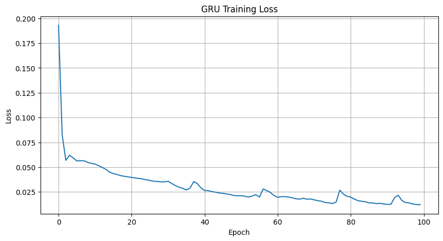
plt.figure(figsize=(10, 5))
plt.plot(gru_train_losses)
plt.title('GRU Training Loss')
plt.xlabel('Epoch')
plt.ylabel('Loss')
plt.grid(True)
plt.show()

Epoch [10/100], Loss: 0.0537
Epoch [20/100], Loss: 0.0401
Epoch [30/100], Loss: 0.0351
Epoch [40/100], Loss: 0.0291
Epoch [50/100], Loss: 0.0211
Epoch [60/100], Loss: 0.0214
Epoch [70/100], Loss: 0.0178
Epoch [80/100], Loss: 0.0206
Epoch [90/100], Loss: 0.0129
Epoch [100/100], Loss: 0.0121

The GRU model shows a clear downward trend in training loss, with a few small blips or fluctuations around epochs 40, 60, 80, and 90. These short-lived spikes are common during training. They can happen when the model momentarily overcorrects as it fine-tunes weights, especially when learning rate adjustments or stochastic variations in batches kick in.

Despite those small bumps, the overall trajectory remains stable, and the final loss value is among the lowest we've seen across all models. This suggests that the GRU was able to settle into an effective pattern of learning and may have captured meaningful structure in the sequence data.

Finally, let's evaluate our GRU model and compare it with the previous ones:

gru_layer.eval()
fc_hidden1.eval()
fc_hidden2.eval()
fc_output.eval()

with torch.no_grad():
    h_0 = init_gru_hidden(len(X_test_tensor))
    gru_out, _ = gru_layer(X_test_tensor, h_0)
    last_output = gru_out[:, -1, :]
    hidden_out1 = F.relu(fc_hidden1(last_output))
    hidden_out2 = F.relu(fc_hidden2(hidden_out1))
    predictions = fc_output(hidden_out2)
    predictions_np = predictions.numpy()
    predictions_original = scaler.inverse_transform(predictions_np)
    gru_r2 = r2_score(y_test_original, predictions_original)

    print("\nModel Comparison:")
    print(f"RNN R²:  {rnn_r2:.2f}")
    print(f"LSTM R²: {lstm_r2:.2f}")
    print(f"GRU R²:  {gru_r2:.2f}")

plt.figure(figsize=(12, 6))
plt.plot(y_test_original, label='Actual Sales')
plt.plot(predictions_original, label='GRU Predictions', alpha=0.7)
plt.title('Cinema Ticket Sales: Actual vs Predicted (GRU)')
plt.xlabel('Day')
plt.ylabel('Total Sales')
plt.legend()
plt.grid(True)
plt.show()

Model Comparison:
RNN R²:  0.51
LSTM R²: 0.58
GRU R²:  0.62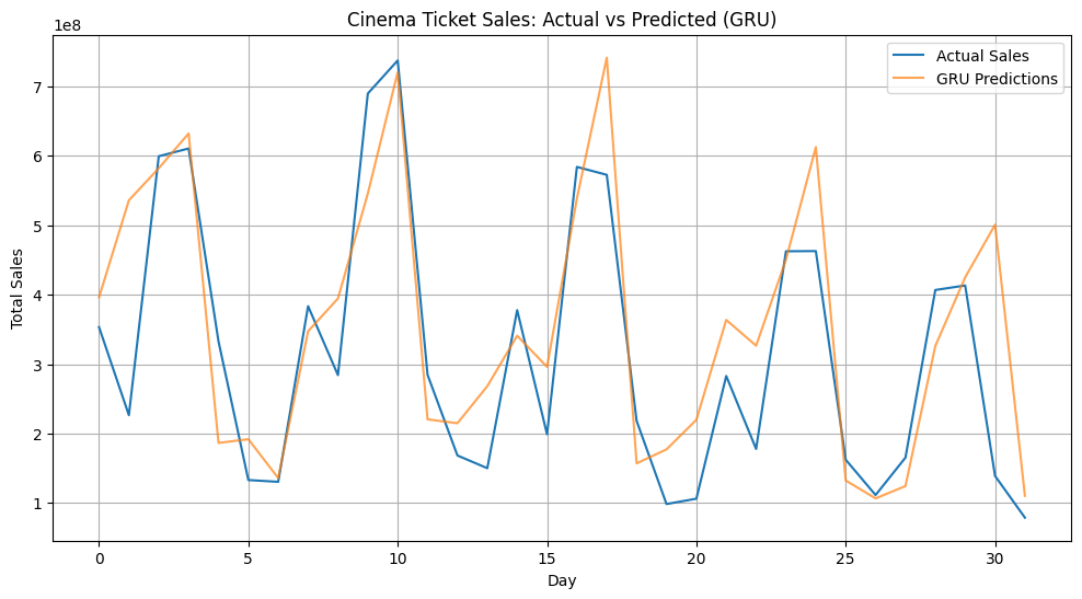

The GRU model finishes strong! Not only did it produce a clean training curve, but it also delivered the highest R² score among the models. While its predictions still miss a few sharp peaks, the GRU tends to follow the overall sales trend more closely and captures weekly patterns with greater consistency.

These results highlight how model architecture affects performance in sequence tasks. The LSTM’s memory cells improved learning over the basic RNN, and the GRU pushed performance even further, offering a nice balance between complexity and accuracy.

While results may vary slightly with different training runs or parameter choices, this progression reflects a common pattern in sequence modeling: adding structure to help the model remember time-dependent patterns typically leads to better outcomes.

Let’s now take a quick look at a few techniques you can use to further improve sequence model performance.

Optimization Techniques for Sequence Models

No model is perfect out of the box. There's almost always room to improve performance through tuning and thoughtful adjustments. In practice, many of the biggest gains come not from completely changing the model architecture, but from small refinements to how the model is trained and optimized.

In this section, we’ll highlight several common strategies that can help your sequence models perform better. We won’t go deep into implementation code here — instead, we’ll walk through the concepts and show simple pseudocode examples to help you understand where and how these techniques fit into your workflow.

1. Adjusting Sequence Length

One of the simplest ways to improve a sequence model is to experiment with the window size — that is, how many previous time steps the model uses to make a prediction. A short window might miss broader trends, while a longer window could introduce noise or unnecessary complexity.

For example:

• A 7-day window can help the model pick up weekly patterns (like weekend sales spikes).
• A 14-day window may capture biweekly or seasonal rhythms.
• Shorter windows (e.g., 3 days) might respond faster to recent trends but miss bigger patterns.

Try testing multiple values and compare performance:

# Pseudocode: test different sequence lengths
for window_size in [3, 7, 14]:
    X, y = create_sequence_data(data, window_size)
    scale → split → train → evaluate
    print(window_size, performance_metrics)

Tuning this one parameter alone can make a noticeable difference in accuracy, especially in time series with strong periodic behavior.

2. Adding Dropout to Prevent Overfitting

If your model performs well on the training set but struggles on the test set, it’s a classic sign of overfitting: the model is memorizing patterns instead of learning general trends.

One common solution is dropout, which randomly disables some neurons during training. This helps the model become more robust by preventing it from relying too heavily on specific pathways in the network.

There are two common places to apply dropout:

• Between recurrent layers (in multi-layer RNNs/LSTMs/GRUs)
• After the recurrent layer, just before the fully connected layers

# Pseudo code: applying dropout
rnn_layer = RNN(..., num_layers=2, dropout=0.2)  # applies dropout between layers
dropout = nn.Dropout(0.2)
x = dropout(recurrent_output)  # applies dropout before output layers

Try different dropout rates (e.g., 0.2–0.5) and compare test set performance. If performance improves without hurting training loss too much, your model was likely overfitting.

3. Using Early Stopping

Even well-designed models can start to overfit if trained for too long. A common solution is early stopping, a simple technique that monitors validation loss during training and stops when performance stops improving.

This prevents wasting time on unnecessary epochs and protects the model from memorizing noise.

# Pseudo code: early stopping
best_loss = float('inf')  # Initialize to a very high value
patience = 10
wait = 0

for epoch in range(num_epochs):
    train()
    val_loss = evaluate_on_validation_set()

    if val_loss < best_loss:
        best_loss = val_loss
        wait = 0
        save_model()
    else:
        wait += 1
        if wait >= patience:
            print("Stopping early")
            break

Early stopping is especially useful when:

• You don’t have a large dataset
• You’ve tuned your model well but still see occasional overfitting
• You want to avoid wasting time or overtraining

Even with just a basic validation split, this technique can make your training more efficient and more reliable.

Takeaways and Recap

We've explored sequence models in PyTorch using cinema ticket sales as our example. Here's what you've learned:

Key Takeaways

• Sequence models help data scientists work with time-dependent data where order matters
• Simple RNNs provide basic pattern recognition but struggle with longer sequences
• LSTM and GRU models solve the vanishing gradient problem, capturing longer patterns
• Data preparation is crucial for sequence models, especially creating time windows
• Optimization through proper sequence length and regularization greatly improves results

Key Terms Recap

• RNN (Recurrent Neural Network): Neural network with recurrent connections that maintain a form of memory about previous inputs
• LSTM (Long Short-Term Memory): Advanced RNN architecture with specialized gates that control information flow, better handling long-term dependencies
• GRU (Gated Recurrent Unit): Streamlined recurrent architecture with fewer parameters than LSTM, often achieving similar performance
• Vanishing Gradient Problem: Issue where gradients become extremely small when backpropagating through many time steps, limiting learning from distant past events
• Sequence Window: Fixed-length segment of sequential data used as input for prediction
• Data Leakage: When information from outside the training set (often from the test set) is accidentally used during training — leading to unrealistically good results and poor generalization

The techniques you’ve explored here form a solid foundation for building smarter models that recognize patterns over time. Whether you're forecasting sales, tracking user behavior, or working with sensor data, sequence modeling is a skill that will serve you well in real-world projects.

Sequence modeling is now part of your toolkit. Keep practicing, keep building.

from Dataquest https://ift.tt/VuHYsU2
via RiYo Analytics