https://ift.tt/qVOmf1E Using Quantum Annealing for Feature Selection in scikit-learn Feature selection for scikit-learn models, for datase...
Using Quantum Annealing for Feature Selection in scikit-learn
Feature selection for scikit-learn models, for datasets with many features, using quantum processing
Feature selection is a vast topic in machine learning. When done correctly, it can help reduce overfitting, increase interpretability, reduce the computational burden, etc. Numerous techniques are used to perform feature selection. What they all have in common is that they look at the set of features and try to separate features that lead to good outcomes (accurate predictions, interpretable models, etc) from features that do not help with this goal.
Particularly difficult are cases where the number of features is very large. An exhaustive exploration of all combinations of features is often computationally prohibitive. Algorithms such as the stepwise search by the regsubsets() function in R may try to infer promising combinations of features by adding / removing features and comparing the results. But ultimately, when the number of features is large, a trade-off remains between the degree of success of the search and the effort spent finding the best combination of features.
As a rule of thumb, when the best solution to a problem involves searching over a large number of combinations, quantum annealing might be worth investigating. I will show an example of feature selection for a dataset with hundreds of features using a scikit-learn plugin recently published by D-Wave.
D-Wave and scikit-learn
Keep in mind, this is not general-purpose, gate-model quantum computing. This is an algorithm that, in essence, is similar to simulated annealing, in that there is an objective function, and something like simulated annealing is used to find a combination of values that minimizes the objective. Except the annealing is not simulated — instead, a real system is programmed such that the physical energy of the system matches the objective function. The energy of the system is lowered until it reaches a minimum (annealing), and then the solution is simply the state of the system, which is read and returned to the user.
D-Wave builds quantum annealers that can efficiently solve many problems where the combinatorial complexity is high. As long as you can reduce the problem to a binary quadratic model (BQM), or a BQM with constraints (CQM), or some discrete generalization of the above (DQM), the problem can be submitted to the quantum solvers. More details are in the documentation.
In theory, you could formulate the feature selection algorithm in terms of a BQM, where the presence of a feature is a binary variable of value 1, and the absence of a feature is a variable equal to 0, but that takes some effort. D-Wave provides a scikit-learn plugin that can be plugged directly into scikit-learn pipelines and simplifies the process.
This article will first show the entire process of explicitly formulating a BQM, then a CQM, sending the model out to the quantum solver, then parsing the results. This is the general method of solving optimization processes on the quantum annealer, and can be used for many problems.
But if all you want is to select the best features in a dataset, a simple SelectFromQuadraticModel() method call is enough. This collapses the whole algorithm into a single line of code. We will show that at the end.
Problem and method
Consider the Scene Recognition Dataset downloaded from OpenML, originally created by Boutell, M., Luo, J., Shen, X., Brown, C. (2004) and distributed under a CC BY license by its authors. It is a binary classification dataset with one dependent variable (Urban), and has nearly 300 features. The value of the response variable (binary: urban or not urban) needs to be predicted based on a combination of features. A simple classification model such as RandomForestClassifier() should perform well, assuming the features are chosen properly.
>>> dataset.get_data()[0]

         attr1     attr2     attr3     attr4     attr5     attr6     attr7     attr8  ...   attr293   attr294  Beach  Sunset  FallFoliage  Field  Mountain  Urban
0     0.646467  0.666435  0.685047  0.699053  0.652746  0.407864  0.150309  0.535193  ...  0.014025  0.029709      1       0            0      0         1      0
1     0.770156  0.767255  0.761053  0.745630  0.742231  0.688086  0.708416  0.757351  ...  0.082672  0.036320      1       0            0      0         0      1
2     0.793984  0.772096  0.761820  0.762213  0.740569  0.734361  0.722677  0.849128  ...  0.112506  0.083924      1       0            0      0         0      0
3     0.938563  0.949260  0.955621  0.966743  0.968649  0.869619  0.696925  0.953460  ...  0.049780  0.090959      1       0            0      0         0      0
4     0.512130  0.524684  0.520020  0.504467  0.471209  0.417654  0.364292  0.562266  ...  0.164270  0.184290      1       0            0      0         0      0
...        ...       ...       ...       ...       ...       ...       ...       ...  ...       ...       ...    ...     ...          ...    ...       ...    ...
2402  0.875782  0.901653  0.926227  0.721366  0.795826  0.867642  0.794125  0.899067  ...  0.254413  0.134350      0       0            0      0         0      1
2403  0.657706  0.669877  0.692338  0.713920  0.727374  0.750354  0.684372  0.718770  ...  0.048747  0.041638      0       0            0      0         0      1
2404  0.952281  0.944987  0.905556  0.836604  0.875916  0.957034  0.953938  0.967956  ...  0.017547  0.019734      0       0            0      0         0      1
2405  0.883990  0.899004  0.901019  0.904298  0.846402  0.858145  0.851362  0.852472  ...  0.226332  0.223070      0       0            0      0         0      1
2406  0.974915  0.866425  0.818144  0.936140  0.938583  0.935087  0.930597  1.000000  ...  0.025059  0.004033      0       0            0      0         0      1

[2407 rows x 300 columns]
A method for choosing the features, described in a paper by Milne, Rounds, and Goddard (2018) is a good fit for the quantum annealers and can be summarized this way:
Split the dataset into the matrix of features, and the response vector — the (X, y) tuple familiar from scikit-learn. Using these, construct a correlation matrix C, where Cii represent the correlations of features with the response, and Cij are the mutual correlations of the features. Of the features that are highly correlated with the response, we want to capture as many as possible. Of the features that are correlated with each other, we want to capture as few as possible, but without affecting features that are strongly correlated with the response. Obviously, we want to strike a balance between all these criteria.
Let Xi be binary variables that indicate whether feature i is chosen for the final dataset. If feature i is chosen, then Xi = 1, otherwise Xi = 0. The problem then becomes equivalent to finding the extreme of:

The first sum of term represents the individual contributions from features — let’s call them linear terms. The second sum of terms could be said to contain quadratic interaction terms. alpha is a bias coefficient that controls the amount of interaction between features that we allow in the objective function; its values will have to be explored to find the best outcome. Finding the set of Xi that minimizes the objective function is equivalent to feature selection.
The objective function is literally a binary quadratic model — BQM. It is binary because Xi can be either 0 or 1. It is quadratic because the highest order terms are the quadratic interactions. This can be eminently solved on a quantum annealer. The only constraint we will need to apply is that the number of variables Xi that are equal to 1 cannot be greater than the total number of features we are willing to accept.
Feature selection the hard way
Let’s solve the problem. The code block below imports all the libraries we need, downloads the dataset, and instantiates a classifier model.
import numpy as np
import openml
from sklearn.ensemble import RandomForestClassifier
from sklearn.model_selection import cross_val_score
import plotly.express as px
from plotly.subplots import make_subplots
import dimod
from dwave.system import LeapHybridCQMSampler

dataset = openml.datasets.get_dataset(312)

X, y, categorical_indicator, attribute_names = dataset.get_data(
    target=dataset.default_target_attribute, dataset_format="dataframe"
)
X = X.astype(float)
y = y.values.astype(int)

clf = RandomForestClassifier()
We are interested in two things:
- the “relevance” of each feature, which is the strength of its correlation with the response
- the “redundancy” of features, which is just the set of non-diagonal items in the correlation matrix (weights of quadratic interaction terms)
Let’s build a couple of functions to visualize relevance and redundancy, apply them to the entire dataset without feature selection, and then cross-validate (5 folds) the performance of the model on the entire dataset.
def evaluate_model(m, X, y, indices=None):
    if not indices is None:
        X_filtered = X.iloc[:, indices]
    else:
        X_filtered = X
    acc = np.mean(cross_val_score(clf, X_filtered, y, cv=5))
    return acc


def show_relevance_redundancy(X, y, indices=None, title=""):
    if not indices is None:
        X = X.iloc[:, indices].copy()
    y = y
    fig = make_subplots(
        rows=1,
        cols=2,
        column_widths=[0.68, 0.32],
        column_titles=["relevance", "redundancy"],
    )
    trace_rel = px.bar(np.array([abs(np.corrcoef(x, y)[0, 1]) for x in X.values.T]))
    trace_red = px.imshow(abs(np.corrcoef(X.values, rowvar=False)))
    fig.add_trace(trace_rel.data[0], row=1, col=1)
    fig.add_trace(trace_red.data[0], row=1, col=2)
    fig.update_layout(width=1200, height=480, title=title)
    fig.show()


show_relevance_redundancy(
    X,
    y,
    None,
    f"full dataset: acc={evaluate_model(clf, X, y, None):.4f}",
)
This is the result:

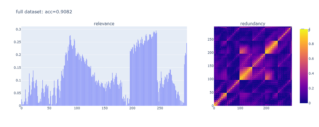
The accuracy of the model is 0.9082. Features vary significantly in terms of relevance. There are pockets of redundancy where there seems to be strong correlation between features.
To minimize the objective function, let’s create a quadratic model with constraints, and send it to the quantum annealer. The code will be explained below.
k = 30
# Pearson correlation
correlation_matrix = abs(np.corrcoef(np.hstack((X, y[:, np.newaxis])), rowvar=False))
# fix the alpha parameter from the Milne paper
# to account for the numerous quadratic terms that are possible
beta = 0.5
alpha = 2 * beta * (k - 1) / (1 - beta + 2 * beta * (k - 1))
# generate weights for linear and quadratic terms, per Milne algorithm
Rxy = correlation_matrix[:, -1]
Q = correlation_matrix[:-1, :-1] * (1 - alpha)
np.fill_diagonal(Q, -Rxy * alpha)
# create binary quadratic model from the linear and quadratic weights
bqm = dimod.BinaryQuadraticModel(Q, "BINARY")
# create constrained quadratic model
cqm = dimod.ConstrainedQuadraticModel()
# the objective function of the CQM is the same as BQM
cqm.set_objective(bqm)
# constraint: limit the number of features to k
cqm.add_constraint_from_iterable(
    ((i, 1) for i in range(len(cqm.variables))), "==", rhs=k
)
# the sampler that will be used is the hybrid sampler in the DWave cloud
sampler = LeapHybridCQMSampler()
# solve the problem
sampleset = sampler.sample_cqm(cqm)
There’s a lot going on there. Let’s explain each step.
We limit the number of features to k=30. This is the main constraint for the model.
We deviate slightly from the objective function described in the paper. Instead of defining alpha directly, we use an equivalent parameter beta, which serves the same purpose. And then we define alpha in a way that keeps the contribution of interaction terms under control — if the number of features is extremely large, this will make sure the interaction terms do not overwhelm the linear terms in the objective function.
We shape the correlation matrix in a way that can be used to build a BQM directly. We constrain the BQM with the condition that no more than k=30 features can be used, and so we obtain a constrained quadratic model (CQM). We send the CQM to the quantum annealer and collect the results.
It should be noted that the run time of the quantum part of the code is about 10 seconds. For many problems, this is a typical baseline duration, even when the number of variables is large. The run time tends to increase with the complexity of the problem, but the increase may not be as abrupt as you’d expect from classical solvers.
We’re not done yet. The D-Wave hardware typically samples the solution space, and returns a large number of potentially feasible solutions. This is due to the way the hardware works: one annealing event is quick and easy to run, so it makes sense to run annealing repeatedly, which is what happens here automatically. If enough samples are generated, some of them will be the best solution.
So we need to sort the solutions and pick the best one. “Best” means — it has the lowest value for the objective function, which D-Wave calls “energy” because it really is the physical energy of the quantum processor.
# postprocess results
feasible = sampleset.filter(lambda s: s.is_feasible)
if feasible:
    best = feasible.first
else:
    assert len(cqm.constraints) == 1
    best = sorted(
        sampleset.data(),
        key=lambda x: (list(cqm.violations(x.sample).values())[0], x.energy),
    )[0]
assert list(best.sample.keys()) == sorted(best.sample.keys())
is_selected = np.array([bool(val) for val in best.sample.values()])
features = np.array([i for i, val in enumerate(is_selected) if val])
best_energy = best.energy
features is the array with the indices of the features picked by the quantum annealer. It is the solution to the feature selection process. Obviously, its length will be k=30.
Let’s measure the accuracy of the model after feature selection:
show_relevance_redundancy(
    X,
    y,
    features,
    f"explicit optimization: acc={evaluate_model(clf, X, y, features):.4f}",
)

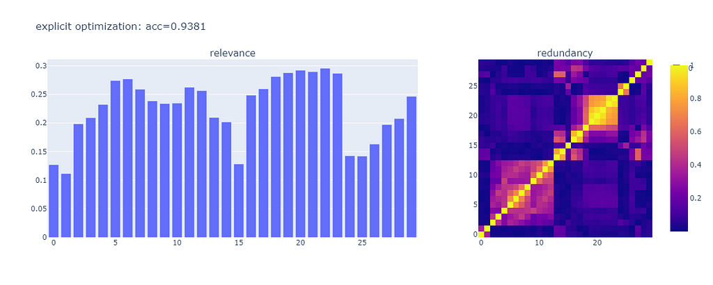
The accuracy of the model after feature selection is 0.9381. We got exactly the number of features we want. Most of them have high relevance. And the correlation values between features are generally low. The model performs better, chances are it’s easier to interpret, and the time it took to select the right features was not too long.
But the process is long and tedious, if all you want is to select some features. Fortunately there is a much easier way now.
Feature selection the easy way
If you have the D-Wave scikit-learn plugin installed, all you have to do is this:
X_new = SelectFromQuadraticModel(num_features=30, alpha=0.5).fit_transform(X, y)
That’s literally it. Behind the scenes, the code creates the quadratic model, constrains it, sends it out to the quantum solver, gets the results back, parses them, and selects the best result to be returned in NumPy array format, the way scikit-learn likes it. The run time is about the same. But let’s see what the results look like:
X_new_df = pd.DataFrame(data=X_new, columns=list(range(X_new.shape[1])))

show_relevance_redundancy(
    X_new_df,
    y,
    None,
    f"plugin optimization: acc={evaluate_model(clf, X_new_df, y, None):.4f}",
)

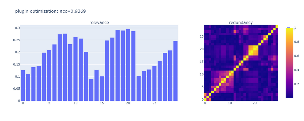
The accuracy of the model is 0.9369, essentially the same as the performance we got from the explicit optimization (well within the typical fluctuation of various random components).
The set of features that got selected is slightly different. This may be accounted for by slight differences between my manual process and the automated implementation in the library.
In either case, we moved the performance of the model up from good to great, with an algorithm that does not guess heuristically, but takes into account the totality of the features.
Further topics to explore
The alpha parameter will bias the feature selection algorithm towards either less redundancy but potentially less quality (alpha=0) or towards higher quality but at the price of increased redundancy (alpha=1). Which is the best value depends on the problem you’re trying to solve.
The SelectFromQuadraticModel() method has a parameter called time_limit which is exactly what the name says: it controls the maximum time spent on the solver. You pay for the time you use, so high values here might be expensive. On the other hand, if the quantum annealing does not seem to converge towards good enough solutions, higher values here might be worth exploring. The problem shown here is rather trivial for the quantum processor, so we just used the default value.
Keep in mind the data exchange between your computer and the quantum solver in the cloud may be non-trivial, so the latency of your connection might be important in time-critical applications such as finance.
References
D-Wave webinar introducing the scikit-learn plugin. https://www.youtube.com/watch?v=VHEpe00AXPI
Milne, A., Rounds, M., & Goddard, P. (2018). Optimal Feature Selection in Credit Scoring and Classification Using a Quantum Annealer. 1QBit.com. https://1qbit.com/whitepaper/optimal-feature-selection-in-credit-scoring-classification-using-quantum-annealer/
Boutell, M., Luo, J., Shen, X., Brown, C. (2004). Learning multi-label scene classification. The Pattern Recognition journal on ScienceDirect. https://www.sciencedirect.com/science/article/abs/pii/S0031320304001074
Getting Started with D-Wave Solvers https://docs.dwavesys.com/docs/latest/doc_getting_started.html
D-Wave scikit-learn Plugin https://github.com/dwavesystems/dwave-scikit-learn-plugin
D-Wave Examples: Feature Selection for CQM https://github.com/dwave-examples/feature-selection-cqm
OpenML Scene Recognition Dataset https://www.openml.org/d/312
Code and artifacts created for this article https://github.com/FlorinAndrei/misc/tree/master/dwave-scikit-learn-feature-selection
Thanks to Dr. Matthew Boutell of the Rose-Hulman Institute of Technology for granting me access to the Scene Features dataset under a Creative Commons license.
All images were created by the author.
Using quantum annealing for feature selection in scikit-learn was originally published in Towards Data Science on Medium, where people are continuing the conversation by highlighting and responding to this story.
from Towards Data Science - Medium
https://towardsdatascience.com/using-quantum-annealing-for-feature-selection-in-scikit-learn-e747d056f673?source=rss----7f60cf5620c9---4
via RiYo Analytics

ليست هناك تعليقات