https://ift.tt/mTNHhtY A hands-on example of how to apply geospatial index Introduction Geospatial Indexing is an indexing technique that...
A hands-on example of how to apply geospatial index
Introduction
Geospatial Indexing is an indexing technique that provides an elegant way to manage location-based data. It makes geospatial data can be searched and retrieved efficiently so that the system can provide the best experience to its users. This article is going to demonstrate how this works in practice by applying a geospatial index to real-world data and demonstrating the performance gain by doing that. Let’s get started. (Note: If you have never heard of the geospatial index or would like to learn more about it, check out this article)
Data
The data used in this article is the Chicago Crime Data which is a part of the Google Cloud Public Dataset Program. Anyone with a Google Cloud Platform account can access this dataset for free. It consists of approximately 8 million rows of data (with a total amount of 1.52 GB) recording incidents of crime that occurred in Chicago since 2001, where each record has geographic data indicating the incident’s location.
Platform
Not only that we’ll use the data from Google Cloud, but also we’ll use Google Big Query as a data processing platform. Big Query provides the job execution details for every query executed. This includes the amount of data used and the number of rows processed which will be very useful to illustrate the performance gain after optimization.
Implementation
What we’re going to do to demonstrate the power of the geospatial index is to optimize the performance of the location-based query. In this example, we’re going to use Geohash as an index because of its simplicity and native support by Google BigQuery.
We’re going to retrieve all records of crimes that occurred within 2 km of the Chicago Union Station. Before the optimization, let’s see what the performance looks like when we run this query on the original dataset:
-- Chicago Union Station Coordinates = (-87.6402895591744 41.87887332682509)
SELECT
  *
FROM
  `bigquery-public-data.chicago_crime.crime`
WHERE
  ST_DISTANCE(ST_GEOGPOINT(longitude, latitude), ST_GEOGFROMTEXT("POINT(-87.6402895591744 41.87887332682509)")) <= 2000
Below is what the job information and execution details look like:
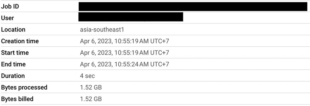

From the number of Bytes processed and Records read, you can see that the query scans the whole table and processes every row in order to get the final result. This means the more data we have, the longer the query will take, and the more expensive the processing cost will be. Can this be more efficient? Of course, and that’s where the geospatial index comes into play.
The problem with the above query is that even though many records are distant from the point-of-interest(Chicago Union Station), it has to be processed anyway. If we can eliminate those records, that would make the query a lot more efficient.
Geohash can be the solution to this issue. In addition to encoding coordinates into a text, another power of geohash is the hash also contains geospatial properties. The similarity between hashes can infer geographical similarity between the locations they represent. For example, the two areas represented by wxcgh and wxcgd are close because the two hashes are very similar, while accgh and dydgh are distant from each other because the two hashes are very different.
We can use this property with the clustered table to our advantage by calculating the geohash of every row in advance. Then, we calculate the geohash of the Chicago Union Station. This way, we can eliminate all records that the hashes are not close enough to the Chicago Union Station’s geohash beforehand.
Here is how to implement it:
- Create a new table with a new column that stores a geohash of the coordinates.
CREATE TABLE `<project_id>.<dataset>.crime_with_geohash_lv5` AS (
  SELECT *, ST_GEOHASH(ST_GEOGPOINT(longitude, latitude), 5) as geohash
  FROM `bigquery-public-data.chicago_crime.crime`
)
2. Create a clustered table using a geohash column as a cluster key
CREATE TABLE `<project_id>.<dataset>.crime_with_geohash_lv5_clustered`
CLUSTER BY geohash
AS (
  SELECT *
  FROM `<project_id>.<dataset>.crime_with_geohash_lv5`
)
By using geohash as a cluster key, we create a table in which the rows that share the same hash are physically stored together. If you think about it, what actually happens is that the dataset is partitioned by geolocation because the closer the rows geographically are, the more likely they will have the same hash.
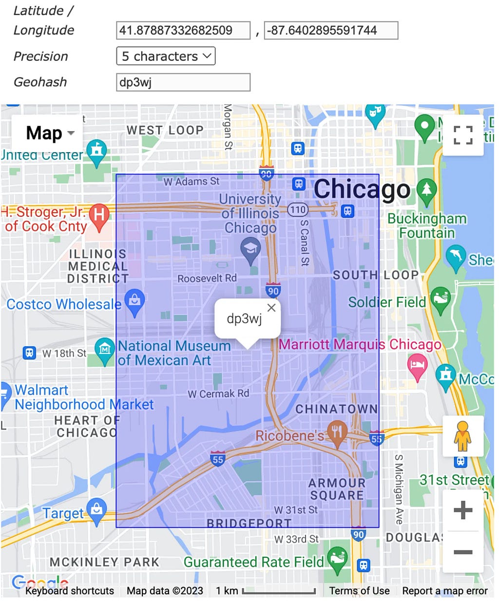
3. Compute the geohash of the Chicago Union Station.
In this article, we use this website but there are plenty of libraries in various programming languages that allow you to do this programmatically.
4. Add the geohash to the query condition.
SELECT
  *
FROM
  `<project_id>.<dataset>.crime_with_geohash_lv5_clustered`
WHERE
  geohash = "dp3wj" AND
  ST_DISTANCE(ST_GEOGPOINT(longitude, latitude), ST_GEOGFROMTEXT("POINT(-87.6402895591744 41.87887332682509)")) <= 2000
This time the query should only scan the records located in the dp3wj since the geohash is a cluster key of the table. This supposes to save a lot of processing. Let's see what happens.
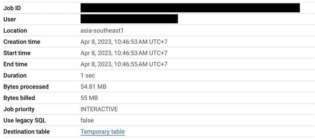

From the job info and execution details, you can see the number of bytes processed and records scanned reduced significantly(from 1.5 GB to 55 MB and 7M to 260k). By introducing a geohash column and using it as a cluster key, we eliminate all the records that clearly do not satisfy the query beforehand just by looking at one column.
However, we are not finished yet. Look at the number of output rows carefully, you’ll see that it only has 100k records where the correct result must have 380k. The result we got is still not correct.
5. Compute the neighbor zones and add them to the query.
In this example, all the neighbor hashes are dp3wk, dp3wm, dp3wq, dp3wh, dp3wn, dp3wu, dp3wv, and dp3wy . We use online geohash explore for this but, again, this can totally be written as a code.
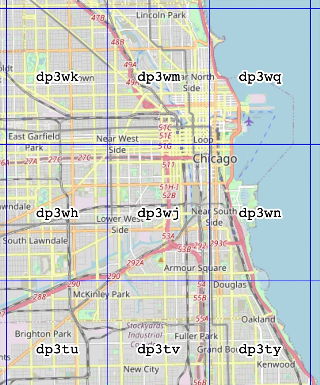
Why do we need to add the neighbor zones to the query? Because geohash is only an approximation of location. Although we know Chicago Union Station is in the dp3wj , we still don't know where exactly it is in the zone. At the top, bottom, left, or right? We have no idea. If it's at the top, it's possible some data in the dp3wm may be closer to it than 2km. If it's on the right, it's possible some data in the dp3wn zone may closer than 2km. And so on. That's why all the neighbor hashes have to be included in the query to get the correct result.
Note that geohash level 5 has a precision of 5km. Therefore, all zones other than those in the above figure will be too far from the Chicago Union Station. This is another important design choice that has to be made because it has a huge impact. We’ll gain very little if it’s too coarse. On the other hand, using too fine precision-level will make the query sophisticated.
Here’s what the final query looks like:
SELECT
  *
FROM
  `<project_id>.<dataset>.crime_with_geohash_lv5_clustered`
WHERE
  (
    geohash = "dp3wk" OR
    geohash = "dp3wm" OR
    geohash = "dp3wq" OR
    geohash = "dp3wh" OR
    geohash = "dp3wj" OR
    geohash = "dp3wn" OR
    geohash = "dp3tu" OR
    geohash = "dp3tv" OR
    geohash = "dp3ty"
  ) AND
  ST_DISTANCE(ST_GEOGPOINT(longitude, latitude), ST_GEOGFROMTEXT("POINT(-87.6402895591744 41.87887332682509)")) <= 2000
And this is what happens when executing the query:
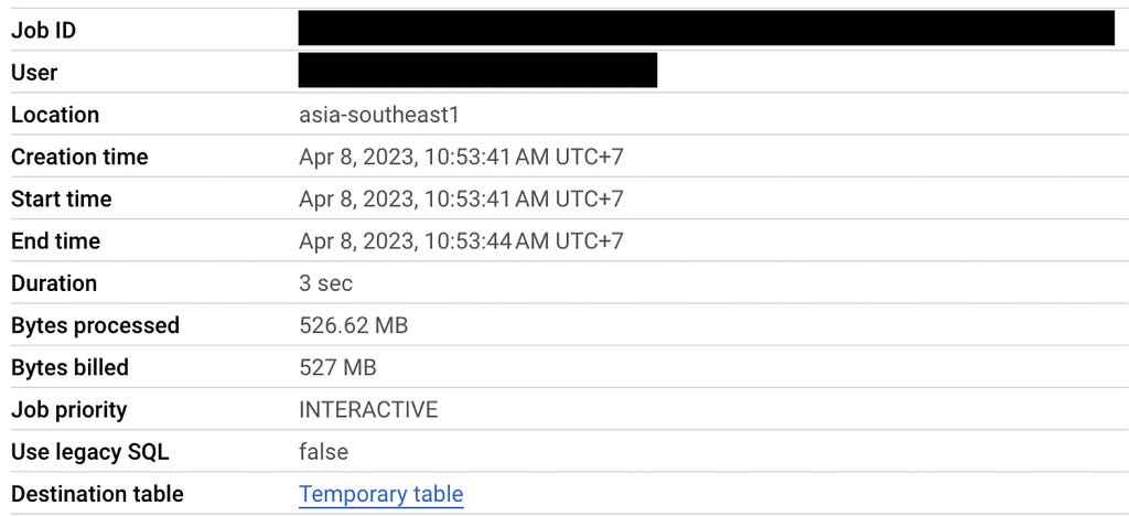

Now the result is correct and the query processes 527 MB and scans 2.5M records in total. In comparison with the original query, using geohash and clustered table saves the processing resource around 3 times. However, nothing comes for free. Applying geohash adds complexity to the way data is preprocessed and retrieved such as the choice of precision level that has to be chosen in advance and the additional logic of the SQL query.
Conclusion
In this article, we’ve seen how the geospatial index can help improve the processing of geospatial data. However, it has a cost that should be well considered in advance. At the end of the day, it’s not a free lunch. To make it work properly, a good understanding of both the algorithm and the system requirements is required.
Originally published at https://thanakornp.com.
Geospatial Index 102 was originally published in Towards Data Science on Medium, where people are continuing the conversation by highlighting and responding to this story.
from Towards Data Science - Medium
https://towardsdatascience.com/geospatial-index-102-cb90c9effb2c?source=rss----7f60cf5620c9---4
via RiYo Analytics

ليست هناك تعليقات