https://ift.tt/T67LAEy Photo by John Matychuk on Unsplash . Parking garages like the one pictured above aim to have every space filled;...

Parking garages like the one pictured above aim to have every space filled; empty spots means unused capacity, which translates to less output in the form of revenue and profit. Similarly, data scientists want their data to have every observation completely filled; missing elements in a dataset translates to less information extracted from the raw data which negatively impacts analytical potential.
Unfortunately, perfect data is rare, but there are several tools and techniques in Python to assist with handling incomplete data. This guide will explain how to:
- Identify the presence of missing data.
- Understand the properties of the missing data.
- Visualize missing data.
- Prepare a dataset after identifying where the missing data is.
Follow the examples below and download the complete Jupyter notebook with code examples and data at the linked Github page.
The Data: Seaborn’s Miles Per Gallon (MPG) Data, Modified
The Python data visualization library Seaborn contains several free, open source datasets for experimentation; learn more about them here. A version of the ‘MPG’ dataset with elements purposefully deleted is available at the linked Github page and will serve as the dataset used throughout this guide.
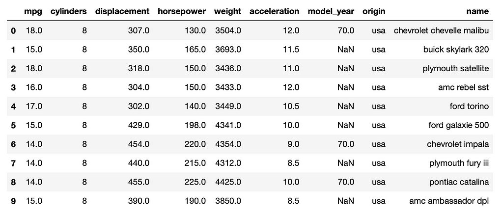
A screenshot of the modified ‘MPG’ dataframe is below — note several “NaN” values in the ‘model_year’ column:
1. Checking for Missing Data
The previous screenshot illustrates the simplest method for finding missing data: visual inspection. This method’s main weakness is handling large data; why look at every row when Python’s Pandas library has some quick and easy commands to rapidly find where the missing data is?
The following code provides a simple starting point to find missing data:
# Load the data into a pandas dataframe:
df = pd.read_csv('mpg-data.csv')
# Display the dataframe's info:
df.info()
This will return:
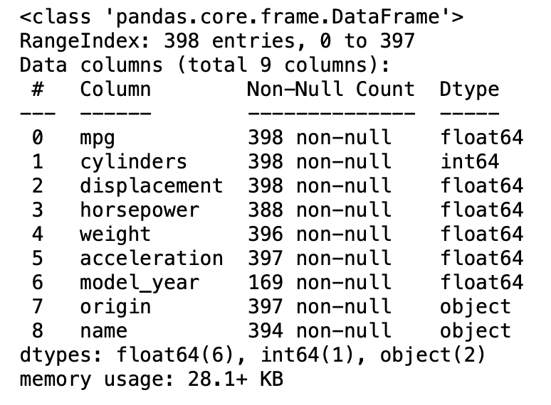
Note that this returns a column titled “Non-Null Count” along with information about the dataframe’s shape (398 entries, 9 columns). The Non-Null Count column shows several columns are missing data, identifiable by their sub-398 non-null count.
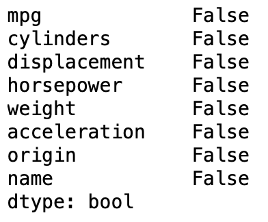
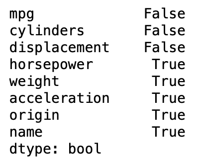
An alternate technique is to run the following code:
df.isnull().any()
The .isnull() function identifies missing values; adding .any() to the end will return a boolean (True or False) column depending upon if the column is complete or not. The above code returns the following:
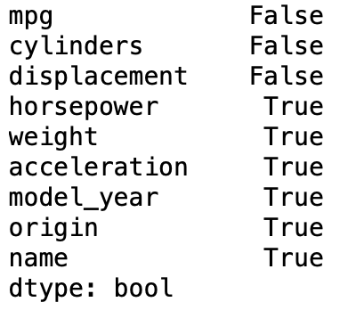
This clearly illustrates which columns contain null (missing) values. Only three columns (mpg, cylinders, and displacement) are complete. Running the same code as above without the .any() returns something different:
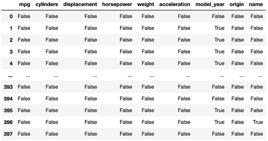
df.isnull()
This returns:
To get a count of null values by column, run the following code.
df.isnull().sum()
This returns:
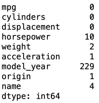
This answers the question of how many missing values are in each column. The following code provides a sum total of all the null values in the entire dataframe:
df.isnull().sum().sum()
The above returns a value of 247.
Another method is to use python’s pandas library to manipulate the outputs of isnull() and use the opposite function, notna(), which returns a count of the filled values in the dataframe. The below code generates a new dataframe that summarizes Null and Not Null values:
# Determine the null values:
dfNullVals = df.isnull().sum().to_frame()
dfNullVals = dfNullVals.rename(columns = {0:'Null'})
# Determine the not null values:
dfNotNullVals = df.notna().sum().to_frame()
dfNotNullVals = dfNotNullVals.rename(columns = {0:'Not Null'})
# Combine the dataframes:
dfNullCount = pd.concat([dfNullVals, dfNotNullVals], ignore_index=False, axis=1).reset_index()
dfNullCount = dfNullCount.rename(columns = {'index':'Category'})
# Display the new dataframe:
dfNullCount
The output of this is:
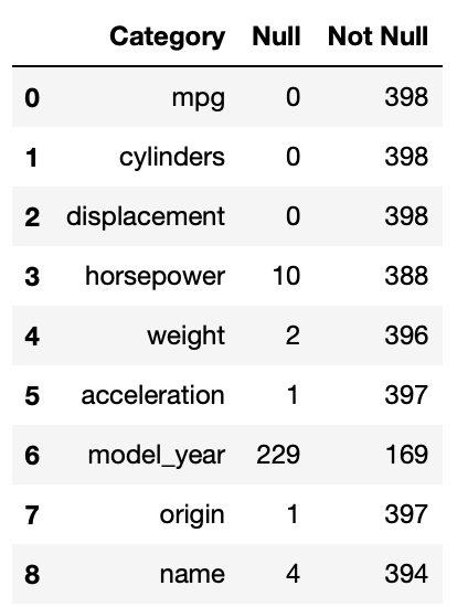
Based on the above code outputs, it is clear the data contains many null values spread across various rows and columns. Some columns are more affected than others. The next step for understanding the missing values is visualization.
2. Visualizing Missing Data
2.1. Missingno Library
Several visualization techniques exist for discovering missing data. One example is missingno. This library is easily installable via:
pip install missingno
Once installed, visualizing missing data is simple. The following code imports the library and displays a bar graph representation of missing data:
import missingno as mi
mi.bar(df)
plt.show()
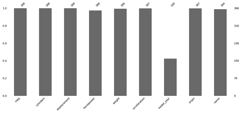
The x-axis shows the columns, while the y-shows the amount filled on a 0 to 1 scale. The totals sit atop the barchart. Note how easy it is to quickly see that over half of ‘model_year’ is missing.
The following code displays another visualization method — the matrix:
mi.matrix(df)
plt.show()
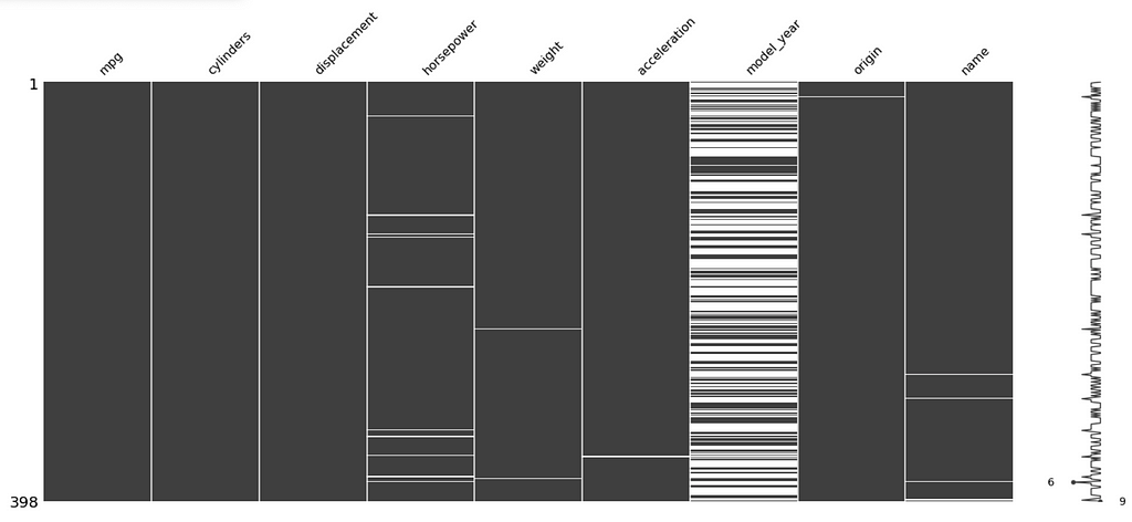
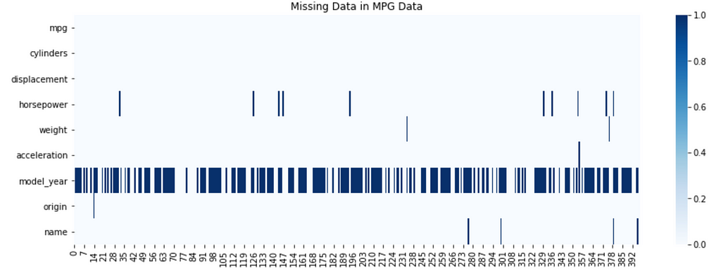
This differs from the bar chart by revealing where missing data resides within each column. The white spaces in each column show missing data; note how ‘model_year’ has a fairly even distribution of missing data throughout the entire column. For further reading on missingno, reference this Towards Data Science article.
2.2. Seaborn Visualizations
Python’s seaborn library offers some easy options for visualization. Specifically, seaborn heatmaps can reveal the presence of missing data, to include where the data occurs spatially within the dataframe. The following code produces a seaborn heatmap:
plt.subplots(figsize=(15,5))
sns.heatmap(df.isnull().transpose(), cmap = 'Blues')
plt.title("Missing Data in MPG Data")
plt.show()
2.3. Plotly
Plotly offers some interactive options for visualizing missing data. Notably, it allows recreating the missingno bar visualization with the option for interactivity and increased customizability.
The first step involves manipulating the data into a dataframe similar to what was done in section one. The second half of the code block creates the bar chart. The code and output are as follows:
# Data Manipulation to Create a Dataframe and Chart Outputting Null and Not Null Value Counts
# Determine the null values:
dfNullVals = df.isnull().sum().to_frame()
dfNullVals = dfNullVals.rename(columns = {0:'Null'})
# Determine the not null values:
dfNotNullVals = df.notna().sum().to_frame()
dfNotNullVals = dfNotNullVals.rename(columns = {0:'Not Null'})
# Combine the dataframes:
dfNullCount = pd.concat([dfNullVals, dfNotNullVals], ignore_index=False, axis=1).reset_index()
dfNullCount = dfNullCount.rename(columns = {'index':'Category'})
# Generate Plot
fig = px.bar(dfNullCount, x="Category", y = ['Not Null', 'Null'])
fig.update_xaxes(categoryorder='total descending')
fig.update_layout(
    title={'text':"Null Values Visualization",
           'xanchor':'center',
           'yanchor':'top',
           'x':0.5},
    xaxis_title = "Category",
    yaxis_title = "Count")
fig.update_layout(legend_title_text = 'Status')
fig.show()
Output:
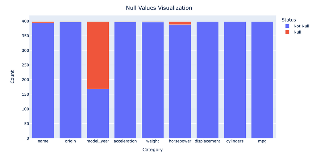
While very similar to what missingno provides, the advantage of the plotly visualization is the customizability and interactivity, to include hoverdata and easily exportable screenshots.
3. What to do with Missing Data?
The final step is determining how to handle the missing data. This will depend upon the problem the data scientist is attempting to answer. From the above visualizations, it is apparent that ‘model_year’ is missing over half its entries, significantly reducing its usefulness.
Under the assumption ‘model_year’ is a useless column, dropping it and creating a new dataframe is simple:
dfNew = df.drop('model_year', axis=1)
Dropping the remaining null values is also simple, requiring just one line of code to create a new dataframe with no null values:
dfNoNull = dfNew.dropna()
# Show if there are any nulls in the new dataframe:
dfNoNull.isnull().any()
Suppose there is value in looking at the columns with null values; creating a dataframe of the incomplete observations is simple:
dfNulls = dfNew[dfNew.isnull().any(axis=1)]
# Show if here are any nulls in the new dataframe:
dfNulls.isnull().any()
The preceding yields two new dataframes: one clear of any missing data, and another containing only observations that have a missing data element.
4. Conclusion
While data scientists will frequently handle incomplete data, there are numerous ways to identify that missing data within a given dataframe. Various visualization techniques aid discovery of null values and assist telling the story of the data’s completeness. Selecting the most appropriate methods to discover, visualize, and handle null data will depend entirely on the customer’s requirements.
References:
[1] Seaborn, Seaborn: statistical data visualization (2022).
[2] M. Alam, Seaborn essentials for data visualization in Python (2020), Towards Data Science.
[3] A. McDonald, Using the missingno Python library to Identify and Visualise Missing Data Prior to Machine Learning (2021), Towards Data Science.
Handling Missing Data in Python was originally published in Towards Data Science on Medium, where people are continuing the conversation by highlighting and responding to this story.
from Towards Data Science - Medium https://ift.tt/UY0gKZu
via RiYo Analytics


No comments