https://ift.tt/7iwtNQG Analyzing Transformers in Embedding Space — Explained How and why look through the embedding space prism Photo by...
Analyzing Transformers in Embedding Space — Explained
How and why look through the embedding space prism

In this post, I present the paper “Analyzing Transformers in Embedding Space” (2022) by Guy Dar, Mor Geva, Ankit Gupta, and Jonathan Berant. Guy Dar is me :)
In this paper, we propose a new method to interpret Transformers by making their parameters more interpretable. We show that some Transformer weights can be “persuaded” to explain what they mean. We use a simple and very efficient technique to translate the model’s weights into tokens. We can translate all weights to vectors and matrices over tokens. Consequently, they are no longer dependent on the model they come from. Then, we can connect different models that use the same tokenizer. Our work relies heavily on Geva et al. (2020, 2022) and Elhage et al. (2021).
Motivation
Transformer models are at the core of NLP and many other subfields of ML. With the growing usability of Transformers comes great responsibility, and people want to know what makes their models tick. Models are often biased (gender, race, …), might be untruthful - feeding off of conspiratorial internet content, and occasionally use abusive language. As more and more sensitive applications use the Transformer, it is crucial to understand its “decision-making” process. This reasoning gave rise to an area of research called interpretability. In an attempt to render models’ outputs more interpretable, researchers have devised many interesting techniques. However, most of them, with a few exceptions, require feeding inputs into the Transformer, and often also computing gradients.
Our method uses only matrix multiplications and does not require example inputs. It can be applied to individual weights rather than all of them at once. The interpretation of a parameter is not restricted to certain inputs as is usually the case for other interpretability techniques. With our method, a parameter is translated from its feature space to another, universal space — the embedding space — where the coordinates are the items of the vocabulary (usually loosely referred to as “tokens”). Since parameters are no longer expressed in the model-specific feature space, but in the common embedding space, we can compare them with parameters in another model, and perhaps even use knowledge from one model in another. We show experiments to support this below.
Terminology
In order to describe our approach accurately, we need to briefly present terminology introduced in previous work.
We follow Geva et al. (2020) and view the FF module as a kind of attention: f(QK^T)V, where Q is the input to the FF module, K are the weights of the first layer of the feedforward module, and V is the weights of the second layer. The difference from the original attention mechanism is that f is GELU instead of softmax, and K and V are input-independent. We call K the FF keys, and V the FF values.
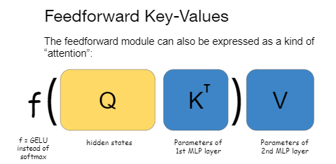
The next concept, which was presented by Elhage et al. (2021), we call the “interaction matrices”. This time we are focusing on the attention module.
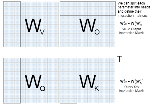
Given an input X to the attention module, we compute Q_att = X W_Q, K_att = X W_K, V_att = X W_V, and then we split them into heads. We could equivalently split the weight matrices into heads in advance, and get the same outcome:

It turns out that the weights of the attention query (W_Q) and key heads (W_K) always operate together — so it makes sense to compute W_QK — the attention query-key matrices:

Now, recall that after concatenating the outputs of all attention heads in the layer, we apply a linear transformation W_O to the concatenated heads. It turns out that each head of the attention value matrix W_V^i always interacts with a certain slice of the attention output matrix W_O — we name it W_O^i. Similar to queries and keys, the value and output heads can be combined into a single matrix per head:

the attention value-output matrices. It is summarized in the following figure:
How to Project Model Parameters?
Embedding space is a central motif in the paper and it is worth discussing it briefly before we continue. Embedding space is a term we use for the vector space where each coordinate corresponds to a vocabulary item (sometimes also referred to as “token”) in the vocabulary of the tokenizer. We differentiate between tokens and vocabulary items, where we consider vocabulary items to be the elements of the vocabulary, and tokens are (potentially duplicate) vocabulary items produced when tokenizing a piece of text. The terms are often used interchangeably by authors, but for clarity, we make a distinction.
Why think of the embedding space? A vector in embedding space can be thought of as representing a weighted sum of words. When we perform operations in embedding space we are actually taking in a “distribution” or scores (they’re not really distributions because they are not constrained to be positive or to sum up to one) over vocabulary items, and output another vector of scores over the items. However, Transformers operate in the latent space (aka feature space), of dense vectors. As a side note, you might feel familiar with operations in the embedding space. Indeed, they are reminiscent of early methods like TF-IDF and bag-of-word classifiers, where scores are obtained from operations directly on tokens.
Can we translate the operation of Transformers in the dense feature space, into operations over vocabulary items in embedding space? We believe the answer is, at least partly, Yes.
The Residual Stream
The residual stream is another concept that appeared in previous work (e.g. nostalgbraist, 2020), and it’s a different view of the layers of the Transformer. The residual stream view stipulates that the model’s hidden states are relatively unchanged between layers, in the sense that the hidden state after the i'th layer is often not very far from the hidden state after the (i+1)’th layer. The reason for that is the residual connection between the layers. The residual connection takes the output of the (i+1)’th layer and adds it to the hidden state after the i’th layer.
As it turns out, the i’th hidden state is usually much more dominant than the vector it is added to — the output of the (i+1)’th layer. This view can be also explained intuitively: the prediction of the next word is usually possible early on in the Transformer, as it usually requires simple reasoning. Some inputs, though, require more complicated processing, and then deeper layers begin to contribute to the final decision.
Instead of thinking in terms of a hidden state per layer, we can think of the hidden states as the residual stream, which is merely slightly updated with every new layer. In a sense, each layer reads from the residual stream and writes into the residual stream, as is visualized in the following figure:
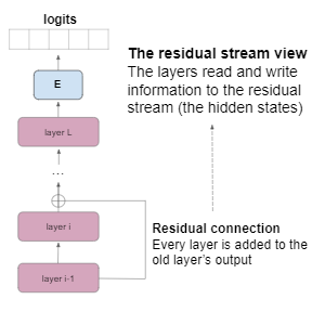
A corollary of this perspective is that, on many occasions, we can ignore the final few layers of the model and get not very different predictions. In some sense, “early exit” is possible in the Transformer.
By extension, we can treat every hidden state as if it were the last hidden state. This is a key observation. What makes it so important? The last hidden state is very significant. In the Transformer, the last hidden state is multiplied by the embedding matrix E and produces the model’s logits — the scores it gives each vocabulary item. If all hidden states are “kind of like the last state”, as we explained above, they can also be projected to the embedding space with E!
Analogously, just like the final hidden state, the projected hidden state produces the logits of the model at this layer of the model! In other words, projecting the hidden state (or residual stream, if you prefer) at layer i gives us the model’s current prediction of the next token.
Geva et al. (2020, 2022) have taken this one step even further and posited that, since FF values are just summed into the hidden states in every layer, perhaps they represent a concept (animals, adjectives, names, etc.) when projected to the embedding space — forming the atoms that the hidden states are made of. They showed empirical results that helped them support this claim.
But one might ask: what about the other parameter groups? attention output is also added to the residual stream, FF keys are interacting with the hidden state from the previous layer. What about W_QK which forms the attention matrix? Can it be translated into a matrix that defines the affinity between vocabulary items? This is what we set out to investigate!
Deriving Other Parameter Projection Schemes
The above techniques we applied to hidden states and FF values can be extended. We use a very simple observation: if h is a hidden state, we can project it to the embedding space with E. Thus, we can think of inner products with h as if they were taking place in the embedding space: h * w = (hE) * (E’ w), where E’ is a right-inverse of E.
So for example, when we compute the interaction between a hidden state h and a FF key, we can re-write this interaction in embedding space. Since hE was identified as the current model’s prediction “scores”, we can think of the inner product as if it decides how much the current prediction corresponds to the concept the key encodes.
This logic can be used to re-interpret the model in the embedding space, where interactions (like hidden states with FF keys) are recast as interactions in the embedding space, and vectors that are added to the residual stream (like FF values) are considered to be interpretable when projecting them with E. We will not elaborate on the entire process. Below, we present a table that summarizes our findings.

As you can see in the table, instead of using an actual right-inverse, we use E’ = E^T even though it’s not a real right-inverse of E. This is because the Penrose-Moore right-inverse, a popular go-to right inverse formula, does not behave well with our interpretation method, for reasons explained in Appendix A of our paper. E^T is actually close enough to be an inverse of the embedding matrix, at least for our purposes. For details — refer to Appendix A of the paper.
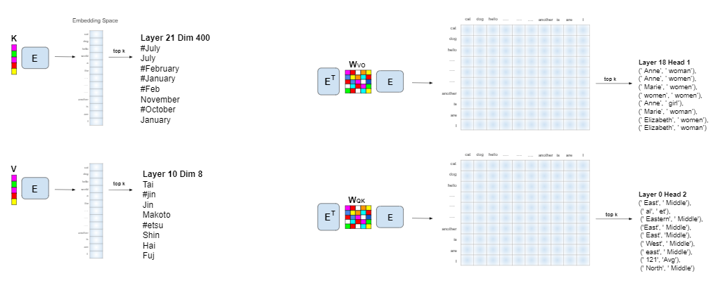
Here’s a schematic overview of our projection to the embedding space:
Examples
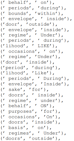
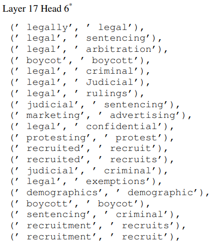
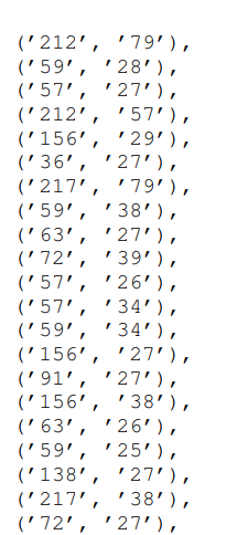
FF keys and values are vectors, and they are projected to vectors in the embedding space. Similarly, W_VO and W_QK are matrices and they are projected to matrices in the embedding space, i.e. they have an entry for every pair of vocabulary items. Since the embedding space is huge, we cannot possibly show all entries when interpreting a vector or matrix. Instead, we choose an integer k and present the top k entries in the vector or matrix.
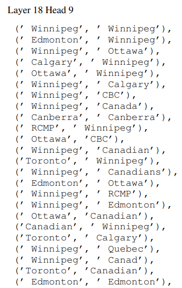
In the following, we show a few interesting examples from the weights of GPT-2 medium. For example, did you know that GPT-2 medium has a Canadian head (in W_VO)?
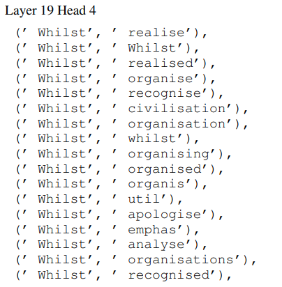
And also a head that speaks British English:
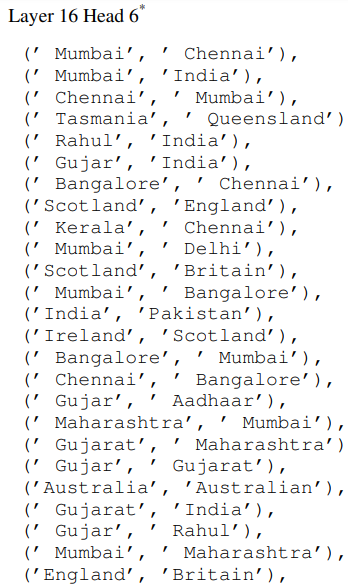
Some more geography:
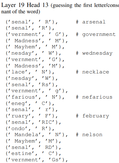
And some very unique heads too:
Also, finding the right preposition is important for fluency:
W_QK has a legal head:
A head for numbers as well:
More is available in Appendix B of our paper!
Applications
Finetuning Directions are Interpretable
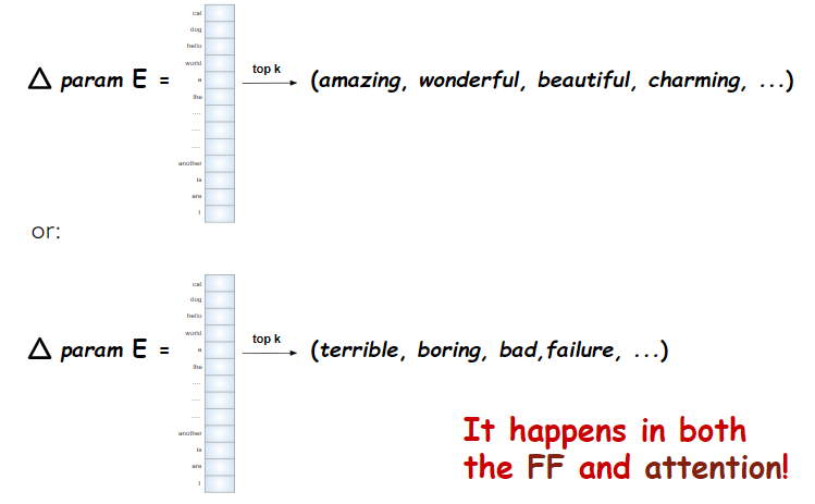
We finetuned a classification head and the last three layers of a pretrained model on IMDB movie reviews (positive or negative review), it turns out that the directions in which parameters move are interpretable. Specifically, the finetuning displacement vectors — the difference between the fine-tuned model’s and the original model’s parameters — are either putting emphasis on tokens related to positive reviews or else emphasizing negative reviews. Schematically:
Next, we show that models learn similar representations in embedding space.
Parameter Alignment Across Models
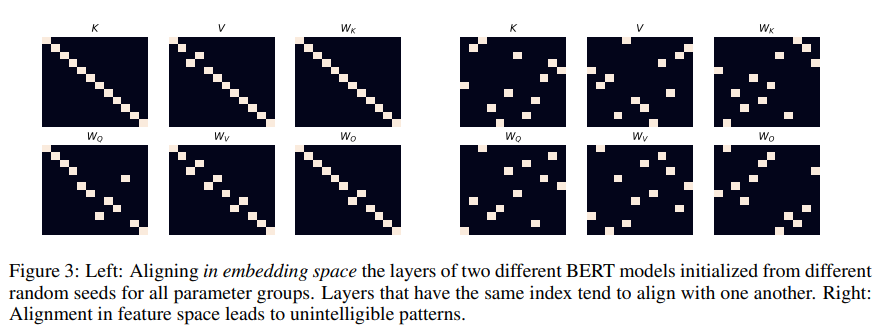
We are using MultiBERTs (Sellam et al., 2022) — which is a collection of BERT models trained on the same data with different random seeds. According to our theory, we can take two separate models and project them both to embedding space. An important observation: since embedding space depends only on the vocabulary, embedding space is shared! Once we’ve projected both models’ parameters into embedding space (each with its own embedding matrix) all parameters lie in the same space. They have a shared language now and we can compare them. When we match parameters from the first model with the second model it turns out that parameters from the same layer are most similar to parameters from the same layer in the other model. This means that layers from both models learn semantically similar concepts in similar layers, but each represents it in its own feature space. While feature space representation is arbitrary and depends on randomness, the embedding space is canonical and stable. That’s why we can compare models in embedding space!
In the following figure we show a comparison between the parameters of two BERTs, both in embedding space (left) and in feature space (right):
Zero-shot Stitching
Think of two models, one pretrained and the other finetuned on a task, say sentiment analysis on IMDB. If we believe that both models operate implicitly in embedding space, we can transfer knowledge from the finetuned model to the pretrained model without any training. We need to translate the feature space of the finetuned model to the feature space of the pretrained model. To do that we take a hidden state in feature space A and project it to embedding space with the help of the embedding matrix of model A, then we project from embedding space to feature space B — using a right inverse of the embedding matrix of model B. This is a simple linear operator that allows us to “switch” feature spaces, and now the finetuned layers from model B can be applied. Pictorially:
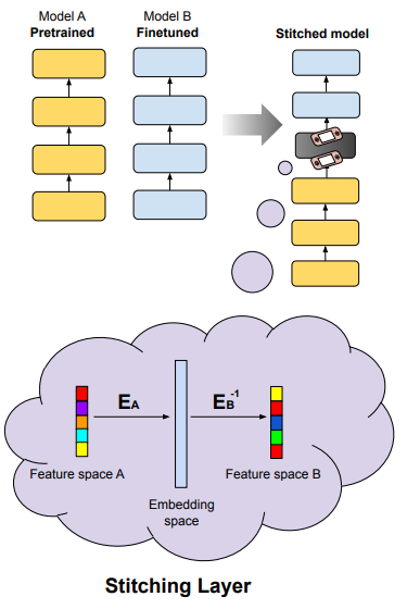
Unfortunately, this does not work as smoothly as expected, and we need to repeat the experiment to obtain good accuracy. It took us 11 runs to get 3 “good” stitched models (with accuracy >70%) on sentiment analysis. Further research would probably resolve this problem. The results are shown in the figure below. The layer axis indicates where in model A we stitched the finetuned layers of model B.

Final Words
We have seen that the Transformer can be viewed as operating in the embedding space, where we can compare different models in a single linear space. We also suggested a new interpretability method for the parameters of a pretrained model. This method does not require feeding inputs to the model and does not require interpreting all the parameters together. We believe that this can lead to many interesting applications in the future. It is important to say that we do not expect our method to be bulletproof. However, we think it is the first step and may serve as a basis for exciting future advancements.
Thanks for reading! Stay tuned!
Please check out our github repo: https://github.com/guyd1995/embedding-space.
If you liked this post you are invited to follow me on twitter: https://twitter.com/guy__dar
All images were created by the author
References
[1] M. Geva, R. Schuster, J. Berant, and O. Levy. Transformer feed-forward layers are key-value memories, 2020. URL https://arxiv.org/abs/2012.14913
[2] M. Geva, A. Caciularu, K. R. Wang, and Y. Goldberg. Transformer feed-forward layers build predictions by promoting concepts in the vocabulary space, 2022b. URL https://arxiv.org/abs/2203.14680.
[3] N. Elhage, N. Nanda, C. Olsson, T. Henighan, N. Joseph, B. Mann, A. Askell, Y. Bai, A. Chen, T. Conerly, N. DasSarma, D. Drain, D. Ganguli, Z. Hatfield-Dodds, D. Hernandez, A. Jones, J. Kernion, L. Lovitt, K. Ndousse, D. Amodei, T. Brown, J. Clark, J. Kaplan, S. McCandlish, and C. Olah. A mathematical framework for transformer circuits, 2021. URL https://transformer-circuits.pub/2021/framework/index.html.
[4] nostalgebraist. interpreting gpt: the logit lens, 2020. URL https://www.lesswrong.com/posts/AcKRB8wDpdaN6v6ru/interpreting-gpt-the-logit-lens.
[5] T. Sellam, S. Yadlowsky, I. Tenney, J. Wei, N. Saphra, A. D’Amour, T. Linzen, J. Bastings, I. R. Turc, J. Eisenstein, D. Das, and E. Pavlick. The multiBERTs: BERT reproductions for robustness analysis. In International Conference on Learning Representations, 2022. URL https://openreview.net/forum?id=K0E_F0gFDgA.
Analyzing Transformers in Embedding Space — Explained was originally published in Towards Data Science on Medium, where people are continuing the conversation by highlighting and responding to this story.
from Towards Data Science - Medium
https://towardsdatascience.com/analyzing-transformers-in-embedding-space-explained-ef72130a6844?source=rss----7f60cf5620c9---4
via RiYo Analytics

ليست هناك تعليقات