https://ift.tt/TkuaVJs Image by SpaceX-Imagery from Pixabay ( License ) We’ll learn how to use the 2SLS technique to estimate linear m...

We’ll learn how to use the 2SLS technique to estimate linear models containing Instrumental Variables
In this article, we’ll learn about two different ways to estimate a linear model using the Instrumental Variables technique.
In the previous article, we learnt about Instrumental Variables, what they are, and when and how to use them. Let’s recap what we learnt:
Consider the following linear model:
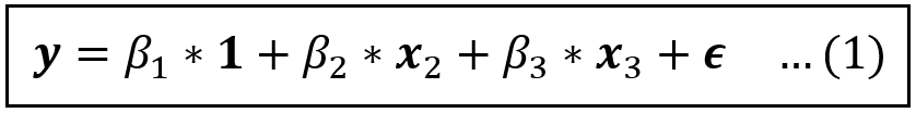
In the above equation, y, 1, x_2, x_3, and ϵ are column vectors of size [n x 1]. From subsequent equations, we’ll drop the 1 (which is a vector of 1s) for brevity.
If one or more regression variables, say x_3, is endogenous, i.e., it is correlated with the error term ϵ, the Ordinary Least Squares (OLS) estimator is not consistent. The coefficient estimates it generates are biased away from the true values, putting into question the usefulness of the experiment.
One way to rescue the situation is to devise a way to effectively “break” x_3 into two parts:
- A chunk that is uncorrelated with ϵ which we will add back into the model in place of x_3. This is the part of x_3 that is in fact exogenous.
- A second chunk that is correlated with ϵ which we will cut out of the model. This is the part that is endogenous.
And one way to accomplish this goal is to identify a variable z_3, “an instrument for x_3”, with the following properties:
- It is correlated with x_3. That (to some extent) satisfies the first of the above two requirements, and
- It is uncorrelated with the error term which takes care of the second requirement.
Replacing x_3 with z_3 yields the following model:
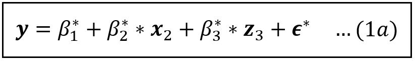
All variables on the R.H.S of Eq (1a) are exogenous. This model can be consistently estimated using least-squares.
The above estimation technique can be easily extended to multiple endogenous variables and their corresponding instruments as long as each endogenous variable is paired one-on-one with a single unique instrumental variable.
The above example suggests a general framework for IV estimation which we present below.
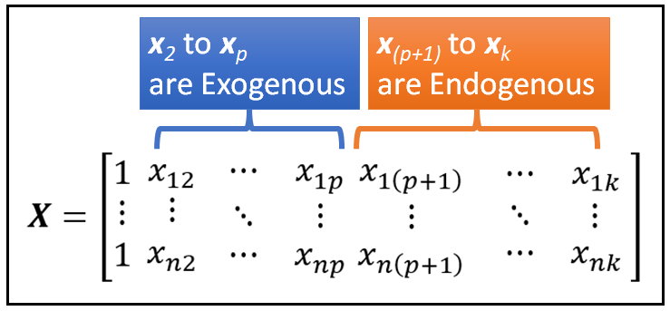
A linear regression of y on X takes the following matrix form:
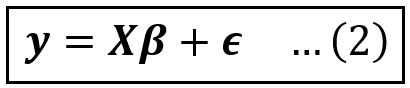
Assuming a data set of size n, in Eq (2):
- y is a vector of size [n x 1].
- X is the matrix of regression variables of size [n x (k+1)], i.e. it has n rows and (k+1) columns of which the first column is a column of 1s and it acts as the placeholder for the intercept.
- β is a column vector of regression coefficients of size [(k+1) x 1] where the first element β_1 is the intercept of regression.
- ϵ is a column vector of regression errors of size [n x1]. ϵ effectively holds the balance amount of variance in y that the model Xβ wasn’t able to explain.
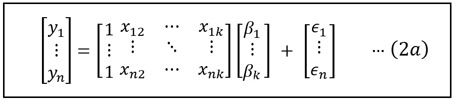
Here’s how the above equation would look in matrix format:
Without loss of generality, and not counting the intercept, let’s assume that the first p regression variables in X are exogenous and the next q variables are endogenous such that 1 + p + q = k:
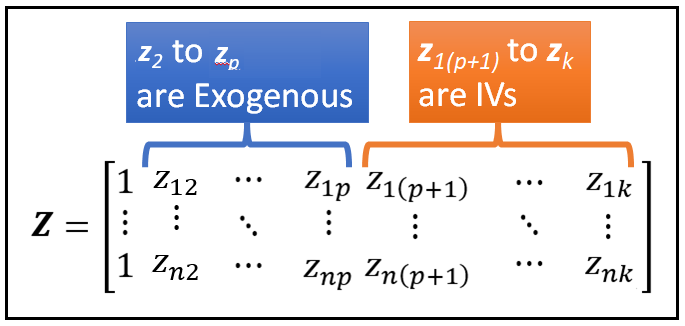
Suppose we are able to identify q instrumental variables which would be the instruments for the corresponding q regression variables in X namely x_(p+1) thru x_k that are suspected to be endogenous.
Let’s construct a matrix Z as follows:
- The first column of Z will be a column of 1s.
- The next p columns of Z namely z_2 thru z_p will be identical to the p exogenous variables x_2 thru x_p in X.
- The final set of q columns in Z namely z_(p+1) thru z_k will hold the data for the q variables that would be the instruments for the corresponding q endogenous variables in X namely x_(p+1) thru x_k.
Thus, the size of Z is also [n x (k+1)] i.e. the same as that of X.
Next, we’ll take the transpose Z which interchanges the rows and columns. The transpose operation essentially turns Z on its side. The transpose of Z denoted as Z’ is of size [(k+1) x n].
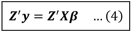
Now, let’s pre-multiply Eq (2) by Z’:
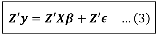
Eq (3) is dimensionally correct. On the L.H.S., Z’ is of size [(k+1) x n] and y is of size [n x 1]. Hence Z’y is of size [(k+1) x 1].
On the R.H.S., X is of size [n x (k+1)] and β is of size [(k+1) x 1]. Working left to right, Z’X is a square matrix of size [(k+1) x (k+1)] and (Z’X)β is of size [(k+1) x 1].
Similarly, ϵ is of size [n x 1]. So Z’ϵ is also of size [(k+1) x 1].
Now, let’s apply the expectation operator E(.) on both sides of Eq. (3):
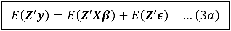
E(Z’y) and E(Z’Xβ) resolve respectively to Z’y and Z’Xβ.
Recollect that Z contains only exogenous variables. Therefore, Z and ϵ are not correlated and hence the mean value of (Z’ϵ) is a column vector of zeros, and Eq (3a) resolves to the following:
Next, we’ll isolate the coefficients vector β on the R.H.S. of (4) by multiplying both sides of Eq (4) with the inverse of the square matrix (Z’X).
The inverse of a matrix is conceptually the multi-dimensional equivalent of the inverse of a scalar number N (assuming N is non-zero). The inverse of a matrix is calculated using a complex formula which we’ll skip getting into.
It is possible to show that (Z’X) is invertible (again something we won’t get into here). Pre-multiplying both sides of Eq. (4) by the inverse of (Z’X) namely (Z’X)^-1, gets us the following:

The yellow and green bits on the R.H.S. cancel each other out and yield an identity matrix in the same way as N*(1/N) equals 1, leaving us with the following equation for estimating the coefficients vector β of the instrumented model:
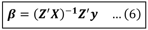
Notice that Z, X and y are all observable quantities and so all regression coefficients can be estimated in one shot using Eq (6) provided there is a one-to-one correspondence between the endogenous variables in X and the chosen instruments in Z.
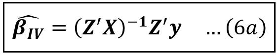
There is one final point that must be mentioned about Eq (6). Eq (6) is strictly speaking estimable only asymptotically, i.e. when the number of data samples n → ∞. But in practice, and for a set of mathematical reasons that probably deserve their own article, we can use it to calculate the coefficient estimates of a model estimated via IV on finite sized samples, in other words, on a real world data set.
Thus, the finite sample IV estimator β_cap_IV of β can be stated as follows:
Now, let’s look at the case where there is more than one Instrumental Variable defined for an endogenous variable.
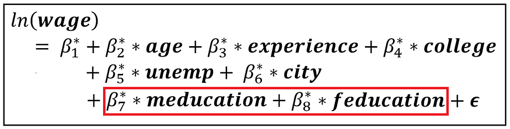
Consider the following regression model of wages:
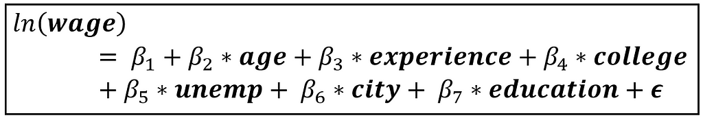
In the above model, we regress the natural log of wage instead of the raw wage as wage data is often right-skewed and logging it can reduce the skew. Education is measured in terms of years of schooling. College and city are boolean variables indicating whether the person went to college and whether they live in a city. Unemp contains the percentage unemployment rate in the county of residence.
Our X matrix is [1, age, experience, college, city, unemp, education], where the each variable is a column vector of size [n x 1] and the size of X is [n x 7].
We’ll argue that education is endogenous. As such, years of schooling captures only what is taught in school or college. And it also leaves out aspects such as how well the person has grasped the material, their knowledge of topics outside of the curriculum and so on, all of which are left unobserved and therefore captured in the error term ϵ.
We’ll propose two variables, mother’s number of years of schooling (meducation) and father’s number of years of schooling (feducation) as the IVs for the person’s education.
The relevance and exogeneity conditions
Our chosen IVs need to pass the relevance condition. If a regression of education on the rest of the variables in X plus meducation and feducation reveals (via an F-test) that meducation and feducation are jointly significant, the two IVs pass the relevance condition.
The error term ϵ is inherently unobservable. So the exogeneity condition for the IVs cannot be directly tested. Instead, we take it upon faith that parents’ number of years of schooling is unlikely to be correlated with factors such as the child’s grasp of material, i.e. the factors that are hiding in the error term and which are making education be endogenous. But we could be wrong about this. We’ll soon find out.
The regression model containing IVs
Our regression model with IVs is as follows:
Our Z matrix is [1, age, experience, college, city, unemp, meducation, feducation], where the each variable is a column vector of size [n x 1] and the size of Z is [n x 8]. Notice how we have replaced education with its two IVs.
And the coefficient vector to be estimated is:
β_cap_IV=[β*_1_cap, β*_2_cap, β*_3_cap, β*_4_cap, β*_5_cap, β*_6_cap, β*_7_cap, β*_8_cap]
Where the caps indicated estimated values.
With X and Z defined, can we use Eq (6a) to perform a single-shot calculation of β_cap_IV?
Unfortunately, the answer is , no.
Recollect that the size of Z is [n x 8]. So, the size of Z’ is [8 x n]. The size of X is [n x 7]. Hence Z’X has size [8 x 7] which is not a square matrix and therefore not invertible. Thus, Eq. (6a) cannot be used when multiple instrumental variables such as meducation and feducation are used to represent a single endogenous variable such as education.
This difficulty suggests that we explore a different approach for estimating β_cap_IV. This different approach is a two-stage OLS estimator.
The 2-stage OLS estimator
We begin by developing the first stage of this estimator.
The First Stage
In this stage, we’ll regress education on age, experience, college, city, unemp, meducation, and feducation.
Let’s suppose that we have determined via the F-test that education is indeed correlated with the IVs meducation and feducation.
We will now regress education not only on meducation and feducation but also the other variables which allows us to account for the effect of possible correlations between the non-IV variables and the IV variables. See my earlier article on Instrumental Variables for a detailed explanation of this effect.
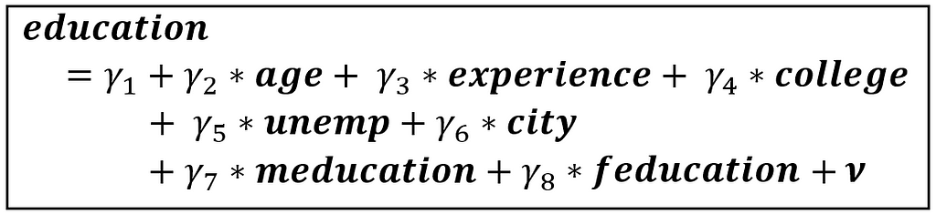
ν is the error term. The above model can be consistently estimated using OLS as all regression variables are exogenous. The estimated model has the following form:
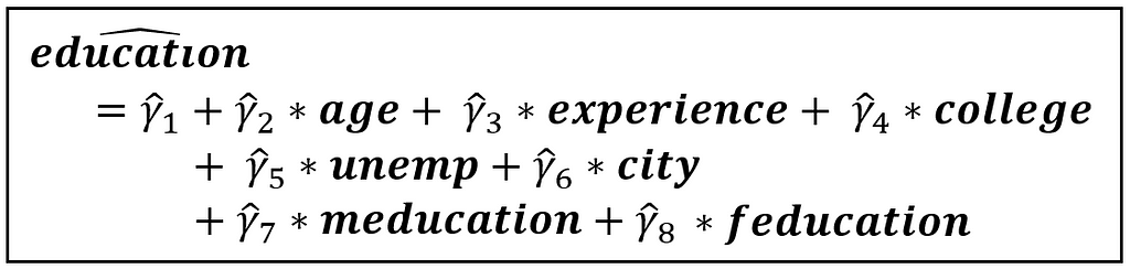
In the above equation, education_cap is the estimated (a.k.a. predicted) value of education. The caps on the coefficients similarly indicate estimated values.
The above OLS based regression represents the first stage of a two-stage OLS (2SLS) estimation that we are about to do.
The second stage
The key insight to be had about the first stage is that education_cap contains only the portion of variance of education that is exogenous, i.e. not correlated with the error term.
Therefore, we can replace education in the original model of ln(wage) with education_cap to form a model that contains only exogenous regression variables, as follows:
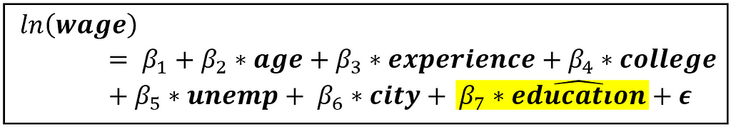
Since the above model contains only exogenous regression variables, it can be consistently estimated using OLS. This estimation forms the second stage of the 2-stage OLS estimator.
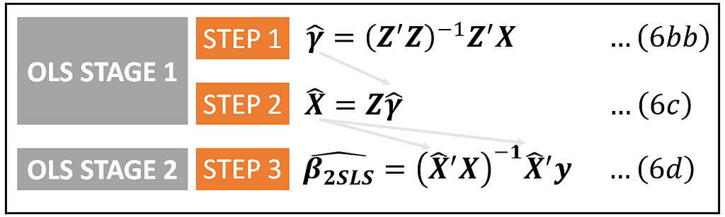
General Framework of 2SLS
For those of you with a flair for linear algebra, the general framework of 2-stage least squares is as follows (if you like, you may skip this section to go straight to the Python tutorial on 2SLS):
Let’s work on the first stage.
Stage 1
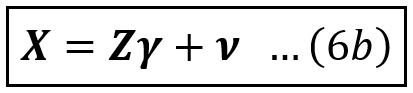
In stage 1, we estimate the following model. To keep things general, X contains not just the endogenous education but also the rest of the variables, γ is the vector of regression coefficients, and ν is the error term:
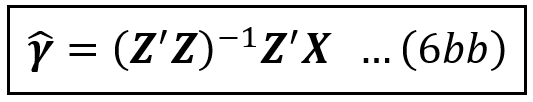
The least-squares estimator of γ can be shown to be calculated as follows using the standard formula for the least-squares based estimator:
Using γ_cap, the estimated value of X is given by:
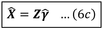
This completes the first stage of 2-SLS.
Now, let’s work on the second stage.
Stage 2
Let’s recollect Eq 6(a) which is the IV estimator we had constructed for the case where there is a one-to-one correspondence between the endogenous variables in X and the instruments in Z:
We’ll plug in X_cap from Eq (6c) in place of Z in Eq (6a) to get β_cap_2SLS as follows:
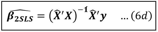
This completes the formulation of the 2-SLS estimator. All matrices on the R.H.S. of Eq (6b) are entirely observable to the experimenter. The estimation of coefficients can be carried out by simply applying equations (6bb), (6c) and (6d) in that sequence:
A tutorial on estimating a linear model using 2SLS using Python and statsmodels
We’ll use the following cross-sectional data from a 1976 Panel Study of Income Dynamics of married women based on data for the previous year, 1975.
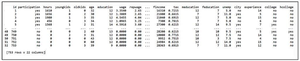
Each row contains hourly wage data and other variables about a married female participant. The data set contains several variables. The ones of interest to us are as follows:
wage: Average hourly wage in 1975 dollars
education: years of schooling of participant
meducation: years of schooling of mother of participant
feducation: years of schooling of father of participant
participation: Did the individual participate in the labor force in 1975? (1/0). We consider only those individuals who participated in 1975.
Our goal is to estimate the effect of education as approximated by number of years of schooling on the hourly wage, specifically log of hourly wage, of married female respondents in 1975.
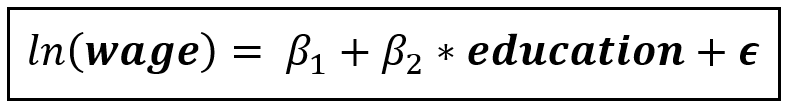
As we saw earlier, education is endogenous, hence a straight-up estimation using OLS will yield biased estimates of all coefficients. Specifically, an OLS estimation of β_1 and β_2 will likely overestimate their values i.e. it will overestimate the effect of education on hourly wages.
We’ll try to remediate this situation by using meducation and feducation as instruments for education.
We’ll use Python, Pandas and Statsmodels to load the data set and build and train the model. Let’s start by importing the required packages:
import pandas as pd
import numpy as np
import statsmodels.formula.api as smf
from statsmodels.api import add_constant
from statsmodels.sandbox.regression.gmm import IV2SLS
Let’s load the data set into a Pandas Dataframe:
df = pd.read_csv('PSID1976.csv', header=0)
Next, we’ll use a subset of the data set where participation=yes.
df_1975 = df.query('participation == \'yes\'')
We’ll need to verify that the instruments meducation and feducation satisfy the relevance condition. For that, we’ll regress education on meducation and feducation, and verify using the F-test that the coefficients of meducation and feducation in this regression are jointly significant.
reg_expr = 'education ~ meducation + feducation'
olsr_model = smf.ols(formula=reg_expr, data=df_1975)
olsr_model_results = olsr_model.fit()
print(olsr_model_results.summary())
We see the following output:
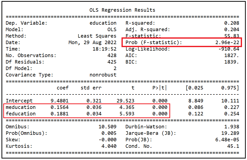
The coefficients of meducation and feducation are individually significant at a p of < 0.001 as indicated by their p-values which are basically zero. The coeffcients are also jointly significant at a p of 2.96e-22 i.e. < .001. meducation and feducation clearly meet the relevance condition for IVs of education.
We’ll now build a linear model for the wage equation and using statsmodels, we’ll train the model using the 2SLS estimator.
We’ll start by building the design matrices. The dependent variable is ln(wage):
ln_wage = np.log(df_1975['wage'])
Statsmodel’s IV2SLS estimator is defined as follows:
statsmodels.sandbox.regression.gmm.IV2SLS(endog, exog, instrument=None)
Statsmodels needs the endog, exog and instrument matrices to be constructed in a specific way as follows:
endog is an [n x 1] matrix containing the dependent variable. In our example, it is the ln_wage variable.
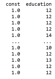
exog is an [n x (k+1)] size matrix that must contain all the endogenous and exogenous variables, plus the constant. In our example, apart from the constant, we do not have any exogenous variables defined in our wage equation. So it will look like this:
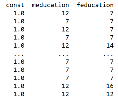
instrument is a matrix that contains the instrumental variables. Additionally, the Statsmodels’ IV2SLS estimator requires instrument to also contain all variables from the exog matrix that are not being instrumented. In our example, the instrumental variables are meducation and feducation. The variables in exog that are not being instrumented is just the placeholder column for the intercept. Hence, our instrument matrix will look like this:
Let’s build out the three matrices:
df_1975['ln_wage'] = np.log(df_1975['wage'])
exog = df_1975[['education']]
exog = add_constant(exog)
instruments = df_1975[['meducation', 'feducation']]
instruments = add_constant(instruments)
Now let’s build and train the IV2SLS model:
iv2sls_model = IV2SLS(endog=df_1975['ln_wage'], exog=exog, instrument=instruments)
iv2sls_model_results = iv2sls_model.fit()
And let’s print the training summary:
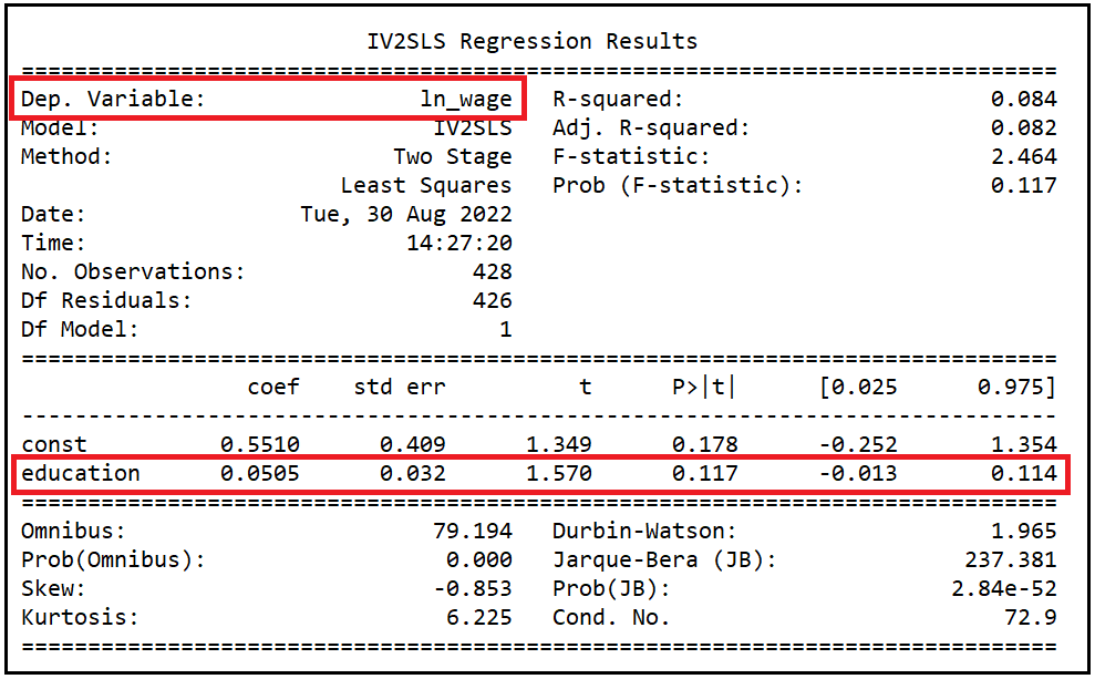
print(iv2sls_model_results.summary())
Interpretation of results of the 2SLS model
Since our primary interest is in estimating the effect of education on hourly wages, we’ll focus our attention on the coefficient estimate of the education variable.
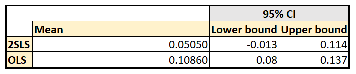
We see that the 2SLS model has estimated the coefficient of education as 0.0505 with a standard error of 0.032 and a 95% confidence interval of -0.013 to 0.114. The p value of 0.117 suggests a significance at (1–0.117)100%=88.3%. Overall, and as expected for a 2-SLS model, the model lacks precision.
Note that dependent variable is log(wage). To calculate the rate of change of hourly wages for each unit change (i.e. one year) of education, we must exponentiate the coefficient of education.
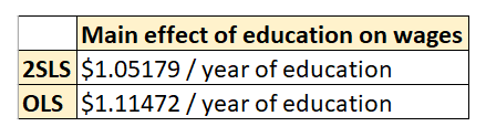
e^(0.0505)=1.05179 implying that a unit increase in number of years of education is estimated to yield an increase of $1.05179 in hourly wages, and vice-versa.
Comparison of the IV estimator with an OLS estimator
Let’s compare the performance of the 2SLS model with a straight-up OLS model that regresses log(wage) on education.
reg_expr = 'ln_wage ~ education'
olsr_model = smf.ols(formula=reg_expr, data=df_1975)
olsr_model_results = olsr_model.fit()
print(olsr_model_results.summary())
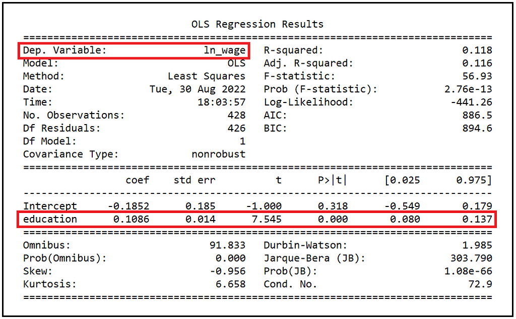
We’ll focus our attention on the estimated value of the coefficient of education. At 0.1086, it is double the estimate reported by the 2SLS model.
e^(0.1086)=1.11472, implying a unit increase (decrease) in the number of years of education is estimated to translate into a $1.11472 increase (decrease) in hourly wages.
The higher estimate from OLS is expected due to the suspected endogeniety of education. In practice, depending on the situation we are modeling, we may want to accept the more conservative estimate of 0.0505 reported by the 2SLS model. However, (and against the 2SLS model), the coefficient estimate from the OLS model is highly significant with a p-value that is essentially zero. Recollect that the estimate from the 2SLS model was significant at only a 88% confidence level.
Also, (and again as expected from the OLS model), the coefficient estimate of education reported by the OLS model has a much smaller standard error (0.014) as compared to that from the 2SLS model (0.032). And therefore, the corresponding 95% CIs from the OLS model are much tighter than those estimated by the 2SLS model.
For comparison, here are the coefficient estimates of education and corresponding 95% CIs from the two models:
With the IV estimator, one trades precision of estimates for the removal of endogeneity and the consequent bias in the estimates.
And here’s a comparison of the main effect of education estimated by the two models on hourly wages:
Data set and tutorial code
The wages data set used in the article can be accessed from this link. The associated documentation can be found here.
Here is the complete source code shown in this article:
Related reading
Introduction to Instrumental Variables Estimation
References, Citations and Copyrights
Data set
The Labor Force Participation data set is available as part of R data sets. It is made available by Vincent Arel-Bundock as part of the Rdatasets package under the GPL-3 license.
Images
All images in this article are copyright Sachin Date under CC-BY-NC-SA, unless a different source and copyright are mentioned underneath the image.
If you liked this article, please follow me at Sachin Date to receive tips, how-tos and programming advice on topics devoted to regression, time series analysis, and forecasting.
Introduction to Two-Stage Least Squares Estimation was originally published in Towards Data Science on Medium, where people are continuing the conversation by highlighting and responding to this story.
from Towards Data Science - Medium https://ift.tt/bzwXra0
via RiYo Analytics


No comments