https://ift.tt/YIQ2dSp Designing a single strategy with 3 datasets—MNIST, Fashion MNIST, and CIFAR 10—to achieve near SOTA accuracy within ...
Designing a single strategy with 3 datasets—MNIST, Fashion MNIST, and CIFAR 10—to achieve near SOTA accuracy within 1000 seconds

This is an experiment where several optimization techniques for faster convergence have been tried for MNIST, Fashion MNIST, and CIFAR 10 dataset, with the only restriction of 1000 seconds on the Google colab provided GPUs. This is helpful when building in-house models or experimenting with a dataset, this technique can be used as base case accuracy.
The main goal is Faster Convergence and a Generalized model. Final result:
Content (step-by-step optimization):
- The Model
- The Data
- The Learning Rate
- Explainability with heatmap
The Model
The first step is to find the right model. The model should have fewer parameters as well as residual properties for faster convergence. There is an online competition about fast training called DAWNBench, and the winner (as of April 2019) is David C. Page, who built a custom 9-layer Residual ConvNet, or ResNet. This model is referred to as “DavidNet”, named after its author. Below is the architecture.
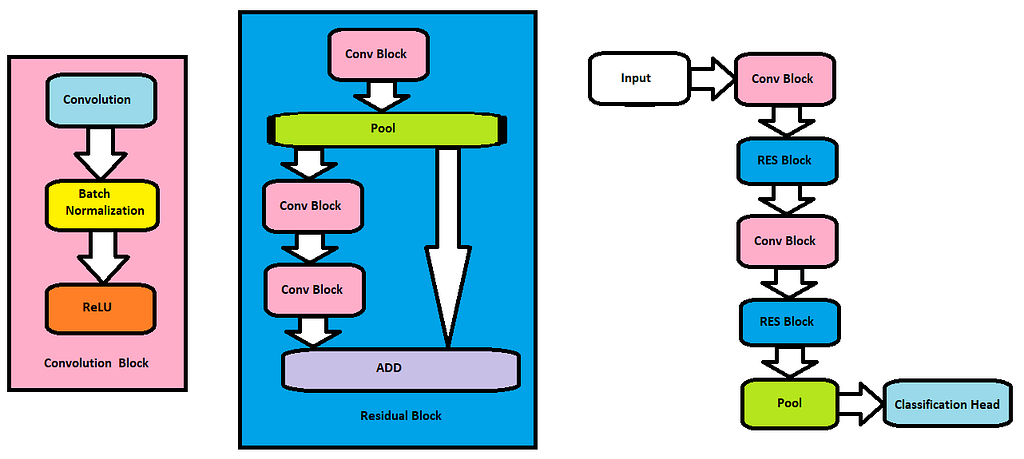
We will use the above model architecture and define it in PyTorch. See the code below.
This model has 6.5 million parameters which is a very small model compared to other larger residual models such as ResNet50 or Vision Transformers.
The model itself will not be enough to achieve high accuracy in a short span of time. We need to optimize the data as well.
The Data
There are 2 optimizations that will be performed with the data.
Augmentation:
- Normalize the Image with the mean and standard deviation of the entire dataset. Normalized Images help in faster convergence.
- Pad the Image that increases 8 pixels in both height and width and then takes a random crop of the image. This helps in creating different x, and y coordinates of the original image.
- Horizontal flip with 50% probability.
- Randomly mask a percentage of Image. Random cutout helps to avoid overfitting.
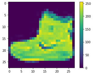
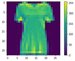
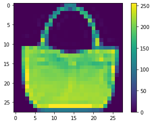
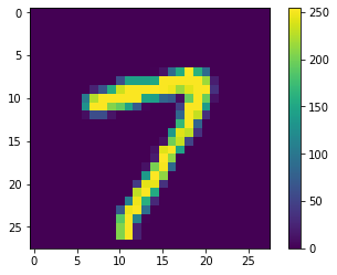
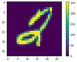
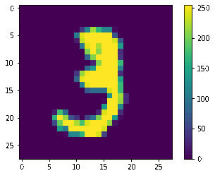
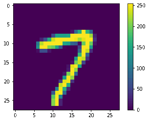
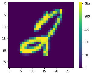
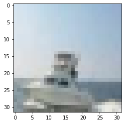
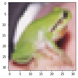
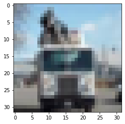
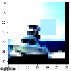
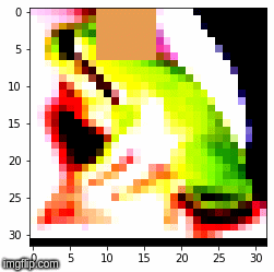
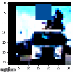
All the above augmentation when applied simultaneously will generate a lot of combinations of images and it is highly unlikely that the model will be trained with the same image with the same orientation in any of the epochs. Below are some examples from all the 3 datasets.
Pre Computation:
The augmentation when applied while training slows down the training process. Say when a batch is to be given to the model, first the augmentation needs to be applied to the Image. During that time the GPU is idle and it is not being utilized to most of its capacity.
Therefore, we will compute all the data augmentations for the number of epochs we plan to train and store all the data variations as tensor flow records. Even when the data is huge, computing augmentation will take time, but once stored as tf records, it can be loaded on the flow from disk without causing any delays.
So with this, we remove the time taken for augmentation from the total training time, which is a significant amount of time. Code below to read and write tf records.
Now, we are done with model and data optimizations. But that still is not enough to achieve the results we desire. We need to optimize one more parameter for faster convergence and that is the optimizer and learning rate scheduler.
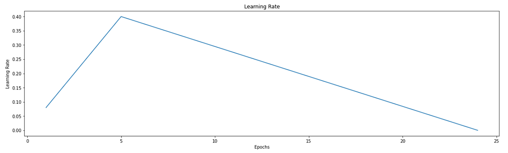
The Learning Rate
We will be using one cycle policy for 25 epochs. Below is the learning rate scheduler graph.
The reason for faster convergence is explained in the below gif.
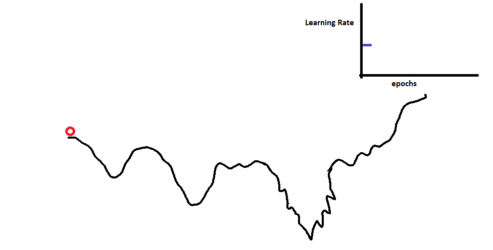
To develop the intuition behind it, we can observe the above gif. The highest accuracy is the lowest possible minima we can find. A constant learning rate will help to find a minima that might not be best. So, to find the best minima we first provide momentum to the algorithm. This will allow it to bounce off the local minima. Then we gradually decrease the learning rate, assuming that at this point in time it is in the global minima section instead of the local minima. Decreasing the learning rate will help it settle down at the bottom as indicated in the gif above.
Now we are all set to train the model and record the time and accuracy.
Training
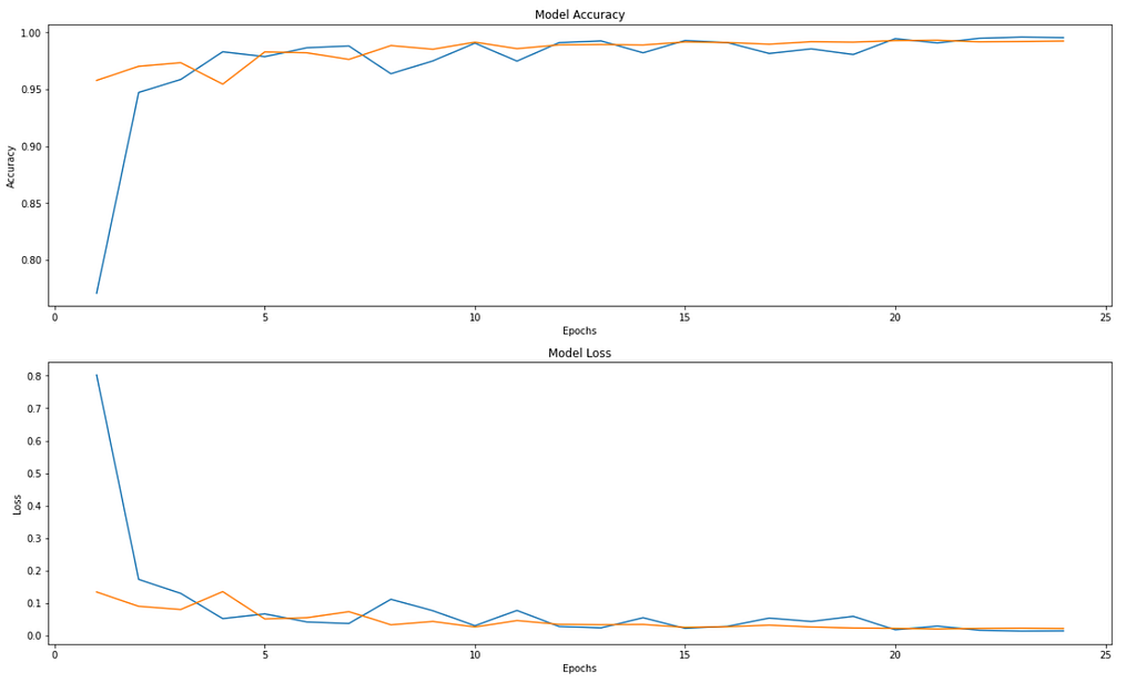
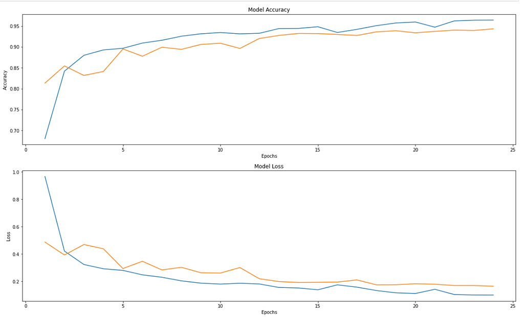
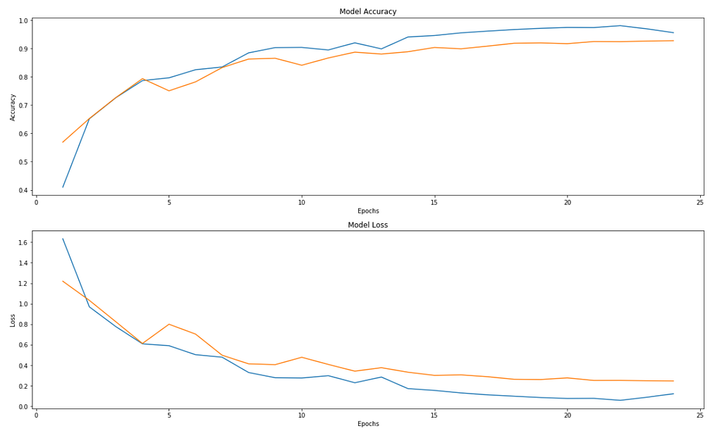
We train for 25 epochs on all the 3 datasets. These are the stats:
We can observe that we are able to achieve very good accuracy that is not very far from SOTA accuracies for all the 3 datasets given the time and resource constraints.
The accuracy and loss graphs for all three datasets are provided below.
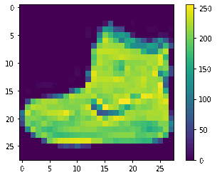
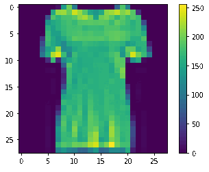
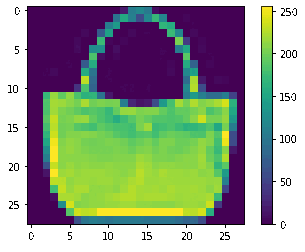
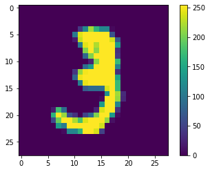
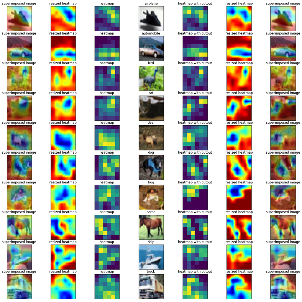
Finally, we also want to know if our model is robust. To do so, we will see the heatmap, by slicing it out of the last few layers to see which part of the image, neurons are more active just before making the predictions.
Explainability with heatmap
In the diagram below, the heatmap of all images run through the trained model is presented for 2 scenarios, one without data augmentation and one with data augmentation. The accuracy is low without data augmentation and as you can see in the diagram below, the model is looking at a more logical section of the image while making predictions when data augmentation techniques are used. Thus making the model more generalized and helping in faster convergence.
The same experiment can be tried with other datasets as well. Although this might not scale for larger datasets with larger image sizes, it will work best for smaller datasets such as those used in this experiment. This can be used as a base case to further optimize and get better accuracy.
In this article, we have explored various techniques for faster training and faster convergence starting with a small but efficient residual network, effective data augmentation techniques that maximize the GPU usage utilization, and one cycle learning rate policy. Combining all this we were able to achieve near SOTA accuracy with publicly available resources within 1000 seconds and 25 epochs. Finally, we evaluate the heatmap to understand the model explainability and whether the model is generalized enough.
Are 1000 Seconds Enough to Train? was originally published in Towards Data Science on Medium, where people are continuing the conversation by highlighting and responding to this story.
from Towards Data Science - Medium https://ift.tt/ID3cnos
via RiYo Analytics


No comments