https://ift.tt/7hRr2yj Understanding adversarial robustness through the lens of convolutional filters Based on collaborative work with Jan...
Understanding adversarial robustness through the lens of convolutional filters
Based on collaborative work with Janis Keuper.
Deep learning has had a significant impact on computer vision. It has enabled computers to automatically learn high-level features from data, and has been used to develop models that can outperform traditional approaches on a variety of tasks such as object recognition, image classification, and semantic segmentation. Applications include autonomous driving, medical diagnosis, and face recognition along many others. However, deep learning models have been shown to be intrinsically sensitive to distribution shifts in the input data.
For example, given sufficiently large and good data, one could easily train a model to recognize street signs (as it would be necessary for autonomous driving tasks). If executed properly, the model will recognize street signs shown during training and ones that is hasn’t been shown previously (it will demonstrate generalization). One could easily conclude that a high validation accuracy would correspond to a model that will safely recognize all new data well. But that often is not the case if there is a distribution shift in the new data. For autonomous driving, this could be due to changes in weather conditions, low-resolution of onboard cameras, poor lighting conditions, etc. that were previously not reflected in training data. I would argue that it is quite impossible to capture training data that will represent all possible environments.
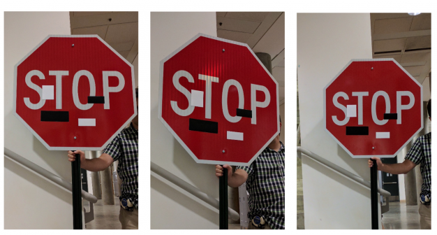
Unfortunately and even worse is that deep learning models have been shown to be even more sensitive: small, for humans barely perceivable perturbations (adversarial attacks) to the input data can force models to make wrong predictions with high confidence. In our previous example, this could mean that a car misclassifies a stop sign for a simple speed limit sign which could have catastrophic consequences. These perturbations are often modeled through noise that is applied to the entire input, but in general, it is also possible to modify small parts of the input, e.g. by placing pieces of tape at a specific location of the street sign to fool models.
A common defense mechanism is a regularization through adversarial training which injects worst-case perturbations back into training to strengthen the decision boundaries and reduce overfitting. However, this technique significantly increases training costs. Therefore, naturally, a deeper understanding of adversarial robustness is of essence to finding better solutions.
While most ongoing research efforts are studying these problems from various angles, in most cases these approaches can be generalized to investigations of the effects of distribution shifts in image data and the resulting differences in activations, saliency-, and feature maps. Instead, we propose to study the shifts in the learned weights (convolution filters) of trained CNN models and ask: What makes the convolutions of robust vision models special?
Evaluation Data & Experiment Setup
To understand differences that arise due to adversarial training we have collected 71 model checkpoints (based on 13 different architectures) from the RobustBench-leaderboard trained on CIFAR-10, CIFAR-100, and ImageNet-1k (robust models). All of these models were trained to withstand L-infinity-bound adversarial attacks based on different approaches, yet, all models were trained with adversarial training. Additionally, we trained an individual model for each appearing architecture using standard training procedures (normal models), without any specific robustness regularization, and without any external data (even if the robust counterpart relied on it). As training on ImageNet1k with our chosen parameters resulted in rather poor performance, we replaced these models with equivalent pre-trained models from the excellent timm-library. In total, we collect 615,863,744 pairs of robust/normal convolution filters of shape 3 x 3.
Filter Pattern Distributions
First, we want to understand the differences in patterns. Since learned filters will be different in magnitude, and, the magnitude is generally lower in deeper layers (to improve gradient flow), we first normalize all filters to unit length. This allows us to focus on the filter pattern without the interference of magnitude. Next, we perform a singular value decomposition (SVD) of all filters. This gives us a representation on a maximum-variance basis: the sum of the 3 x 3=9 principal components (also called basis vectors or eigenimages) weighted by the 3 x 3=9 coefficients allows the reconstruction of every filter.

This gives us the advantage, that the representation on the SVD-obtained basis is not limited to individual pixels but captures relevant subpatterns of the filter (refer to v0 … v9). To analyze multiple filters we can simply treat coefficients on the same basis as distributions.

To measure how different two distributions Pi, Qi are, we can use any divergence measurement. In this work, we use the well-known Kullback-Leibler divergence (KL) with a minor tweak to enforce symmetry.

For each set of filters, we obtain 9 distributions. In order to compare two filter sets, we compute the KL on every basis vector and compute a weighted mean. The weight of each basis vector is given by its variance ratio. In the following sections, we refer to this as a distribution shift.
Note: In our previous work [2] saw a hefty impact of sparse filters on the distributions. Sparse filters will be mostly described by near-zero coefficients that will result in large spikes in the KDEs. The KL divergence will be heavily increased and biased to this region of the KDEs. Therefore, we remove sparse from layer weights for this analysis.
Where are the largest distribution shifts located?
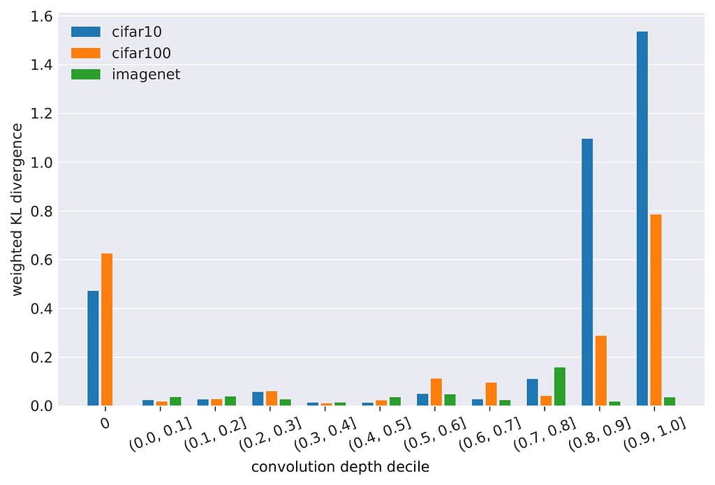
We investigate the most significant shifts in filter patterns and measure the distribution shift at various stages of depth. To compare models with different depths, we group filter coefficients in deciles of their relative depth in the model. For all datasets, the obtained shifts seem to increase with convolution depth. However, the difference decreases with dataset complexity (ImageNet1k > CIFAR100 > CIFAR10). Additionally, a significant shift can be seen in the very first convolution layer (but not the following early layers). Please note that the primary convolution stages in ImageNet1k-models use a larger kernel size and are therefore not included in this study, yet we expect similar observations there. Image by the authors.
In order to better understand the cause of the observed distribution shifts, we visualize the first and last (ultimate) convolution layers:


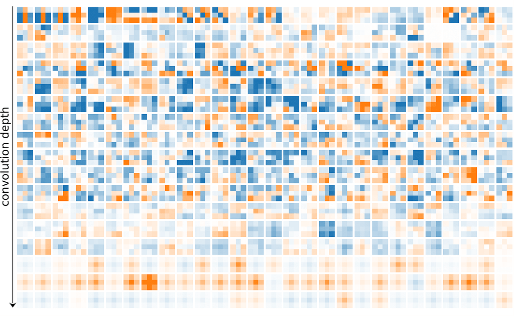
For the deepest convolution layers, we observe that normal filters show a clear lack of diversity, and mostly remind us of gaussian blur filters, while adversarially-trained filters appear to be richer in structure and are more likely to perform less trivial transformations. We observe this phenomenon in many of the deeper layers.


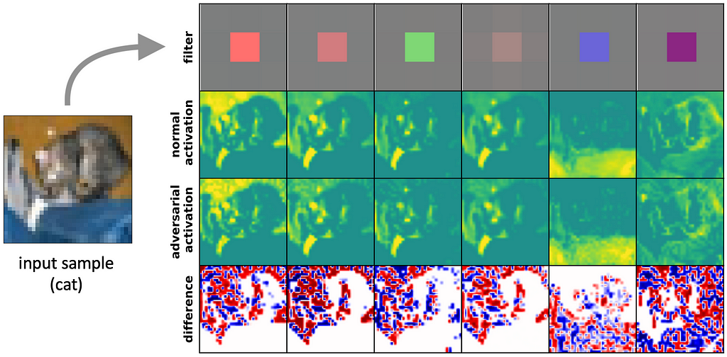
On the other hand, the primary convolution stage shows a striking opposite that we seldomly find in other layers: Normal models show an expected diverse set of various filters, yet, all robust models develop a large presence of highly similar filters. Since only their center weight is non-zero, these filters are performing a weighted summation of the input channels equivalently to 1 x 1 convolutions.
We hypothesize that in combination with the commonly-used ReLU-activations (and their derivatives) the primary filters perform thresholding of the input data which can eliminate small perturbations. Indeed, plotting the difference in activations for natural and perturbed samples, allows us to obtain visual confirmation that these filters are successful in removing perturbations from various regions of interest (ROI), e.g. from the cat, background, and foreground. It seems like adversarially-robust models are not intrinsically robust but learn to preprocess the data.
What differences do we observe in filter quality?
We can also think of what properties “good” convolution filters would have: In order to utilize as much as possible of the learned network, all filters in a convolution layer should contribute to predictions, and the patterns in a layer should in general not be too repetitive and produce diverse feature maps.
We measure the quality through three different static metrics (meaning by only using learned parameters):
Sparsity — the ratio of non-contributing filters
The ratio of filters where all weights are near-zero sparsity in a given layer. These filters do not contribute to the feature maps due to their low magnitudes. To maximally use the available network capacity, this value should be as low as possible.
Variance entropy — the diversity of filter patterns
We exploit SVD again to understand the diversity of patterns in a given layer. As the SVD finds the maximum variance basis, it will naturally identify the most important “sub-patterns”. By capturing the distributions of explained variance we can identify whether a single sub-pattern is dominant (lack of diversity; skewed variance distribution) or all sub-patterns are equally important (random/maximum diversity; uniform variance distribution). We quantify the distribution of explained variance by the non-negative log entropy. An entropy variance value of 0 indicates a homogeneity of present filters, while the maximum indicates a uniformly spread variance across all basis vectors, as found in random, non-initialized layers. Values close to both interval bounds indicate a degeneration, and, it is difficult to provide a good threshold.
Orthogonality — the redundancy of filterbanks/resulting feature maps
Orthogonality helps with gradient propagation and is directly coupled with the diversity of generated feature maps. Due to computational limits, we measure the orthogonality between filterbanks instead of individual filters. The filterbanks are treated as vectors and are normalized to unit length. The orthogonality is then simply the dot product between the layer weight and its transpose. An orthogonality value of 1 stipulates the orthogonality of all filterbanks in a layer, whereas 0 indicates parallel filterbanks that produce perhaps differently scaled but otherwise identical feature maps.
Eventually, all these three metrics quantify the amount of used capacity concerning the network size.
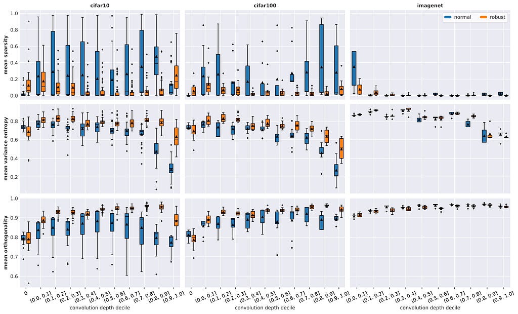
Similar to the findings in structure, we observe fewer differences in quality with dataset complexity, but also a general increase in quality for both robust and normal models. The results on ImageNet1k are less conclusive due to a low sample size and a near-optimal baseline in terms of quality
Sparsity: We observe a very high span of sparsity across all layers for normal models that decreases with dataset complexity. Robust training significantly further minimizes sparsity and its span across all depths. Notable outliers include the primary stages, as well as the deepest convolution layers for CIFAR-10. Generally, sparsity seems to be lower in the middle stages.
Variance entropy: The average variance entropy is relatively constant throughout the model but decreases with deeper layers. The entropy of robust models starts to decrease later and is less significant but the difference diminishes with dataset complexity. Compared to CIFAR-10, robust CIFAR-100 models show a lower entropy in deeper layers, while there is no clear difference between normal models. ImageNet1k models show a higher entropy across all depths.
Orthogonality: Robust models show an almost monotonic increase in orthogonality with depth, except for the last decile, whereas normal models eventually begin to decrease in orthogonality. Again the differences diminish with dataset complexity and the span in obtained measurements of non-robust models is crucially increased.
Conclusion
Adversarially-trained models appear to learn a more diverse, less redundant, and less sparse set of convolution filters than their non-regularized variants. We assume that the increase in quality is a response to the additional training strain, as the more challenging adversarial problem occupies more of the available model capacity that would otherwise be degenerated. We observe a similar effect during normal training with increasing dataset complexity. However, although the filter quality of normally trained ImageNet1k models is comparably high, their robustness is not. So, filter quality alone is not a sufficient criterion to establish robustness.
Next Steps
Unfortunately, we weren't able to fully demystify the impact of adversarial training on convolution filters. In particular, it remains unclear if dataset complexity is the cause for lower quality shifts, or if the difference in quality that we measure is merely a side effect of heavily overparameterized architectures in which adversarial training can close the gap to more complex datasets. It appears as if more analysis is necessary to fully grasp the impact of adversarial training, and, it is very likely that there are other mechanics in play that lead to robust models. On the other hand, filter quality seems to at least be a necessary condition to achieve robustness. Therefore it seems worthwhile to explore if we can increase robustness by enforcing higher filter quality during training through regularization. Perhaps, this could even become a cheaper replacement for adversarial training.
What do you think? We are curious about your thoughts! Please share them in the comments.
References:
[1] P. Gavrikov and J. Keuper, Adversarial Robustness Through the Lens of Convolutional Filters (2022), CVPR 2022 Workshops
[2] P. Gavrikov and J. Keuper, CNN Filter DB: An Empirical Investigation of Trained Convolutional Filters (2022), CVPR 2022 Orals
This work was funded by the Ministry for Science, Research and Arts, Baden-Wuerttemberg, Germany under Grant 32–7545.20/45/1 (Q-AMeLiA).
What Makes the Convolutions of Robust Vision Models Special? was originally published in Towards Data Science on Medium, where people are continuing the conversation by highlighting and responding to this story.
from Towards Data Science - Medium https://ift.tt/uJkrqxd
via RiYo Analytics

No comments