https://ift.tt/JT5lW69 Applying convolution and attention mechanism on graphs An aesthetic network, picture by Alina Grubnyak In the la...
Applying convolution and attention mechanism on graphs

In the latest years, Graph Neural Networks are quickly gaining traction in the Machine Learning field, becoming suitable for a variety of tasks. It’s no doubt that the advent of Social Networks played an important role in GNNs’ success, yet they turned out to be applicable also in biology, medicine, and other fields where graphs represent the fundamental entity.
I’m always attracted by arising technologies and methodologies, hence why I decided to give it a shot and learn something about it. Furthermore, to let the knowledge settle, I decided to write this post to put down all the concepts I bumped into in this journey of mine.
Methodically organizing all the content may be useful for a quick review in the future, or hopefully serve someone else in need of a learning resource.
Enough talk for now, let’s start from the fundamentals!
What is a graph?
If you are reading this post, you’ll most likely already know what a graph is, so I won’t be long on this.
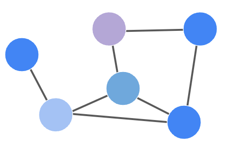
A graph is a structure G composed of nodes V, connected between them by edges E.

Nodes can have features, that better describe the node itself. For instance, if nodes represent people, their features could be age, sex, height, and more.
Edges between nodes represent relationships, namely two nodes are connected if they have a relationship (think of the concept of follows on Instagram), and they can be undirected, if the relationship is symmetric, or directed if the relationship is not symmetric.
As I said, I’m not going deeper on this, because it’s not in the scope of the article, yet I needed to introduce some terminology for the sake of the read.
Introduction to Graph Neural Networks
Given that graph structures are so abundant in our daily lives (social networks, maps, user-product interactions …), researchers started the hunt for a Deep Learning architecture capable of dealing with them. In the last 10 years of DL research, Convolutional Neural Networks became one of the most fortunate architectures, which work on a particular example of graphs: images.
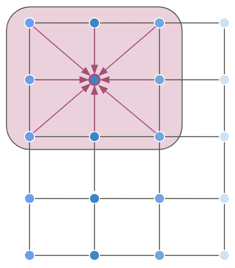
Images can be thought of as a special case of graphs, where pixels represent nodes organized in a grid, and their greyscale/RGB value are their features.

When you apply convolution on a set of pixels, you are summarizing the information gained from the pixel where the convolution is centered, combined with all of its neighbors.
Now, you cannot directly apply convolution on graphs, because graph nodes do not have an inherent ordering (differently from images, where pixels are uniquely determined by their coordinates in the image).
So researchers wondered: can we generalize the convolution operation on graphs?
They came out with two classes of methods:
- Spectral methods: as you may guess from the name, they have something to do with the frequency domain. They preserve the strict concept of convolution, yet they are a bit tricky to understand. Despite being more mathematically sound, they are rarely used due to their computational cost.
- Spatial methods: they represent a decent approximation of spectral methods, despite not being as mathematically strict. Easier to understand, they are based on the concept that every node should collect information from itself and its K-hops neighbors.
Personally, I had a look at spectral methods, but since they are not the most used today, I decided not to give them too much space, in favor of spatial methods, which I’ll cover more in this post.
Here we go: Graph Convolutional Networks
The first successful example of Deep Learning and convolution application on graphs was presented in Kipf & Welling, 2017, where Graph Convolutional Networks were introduced.
The main idea behind their algorithm is the following:
- You apply a linear projection to all the feature vectors of your nodes
- You aggregate them (mean, sum, concat…)
- You combine the projection of a node together with its neighbors’ projections.
Here’s the process in formulae:


Equation 1 is the mathematical expression of the steps listed before. The embedding of each node is obtained by projecting each neighbor into another space, averaging (but other types of aggregation can be used), and combining them with the projection of the node itself. The last step, as usual in DL, is the activation function pass.
This is brilliant, isn’t it? However, while I was reading it, I was a bit puzzled about how you code this. Ok, I have a graph, but how do I efficiently find the neighbors of each node, in order to combine their features? Easy, you use the adjacency matrix A!
The adjacency matrix A, whose size is N² (N is the number of nodes), describes how nodes are connected: A(v,u) = 1 if nodes v, u are connected.
For instance, if you simply want to aggregate the features of all the neighbors (a.k.a. 1-hop nodes) of a node you just do:


Now, if you keep iterating this process over k-steps, you aggregate features from k-hops neighbors, and the expression above can be easily expressed as follows, where the linear projection has been added:

Note that the original paper does not use the plain adjacency matrix A. The authors apply some normalization tricks which improve performance, but for the sake of learning this is enough to understand the concept.
Therefore the parameter k regulates both the number of layers and the number of hops that you want to learn from. This is something not super obvious and quite smart! But… how should I choose k?
A peculiar element of GCNs is that they are usually not deep networks, instead, they are more likely very shallow (most of the times 2 layers are enough!). As of today, it’s not evident why shallow networks work better, but here’s some intuition behind it:
- if the network is strongly connected, a single node can reach most of the others in just a few hops
- many learning tasks rely on the assumption that information from close nodes is more relevant than remotes’
This is cool, right? It looks like a few layers (and hence parameters) do the trick! Well, yes, but GCNs usually cope with scalability problems due to graphs’ size. Think of applying Equation 3 on a graph with millions of nodes: the adjacency matrix would be huge! Fortunately, there are papers exploring learning techniques on such large graphs, such as GraphSAGE.
What can you do with GCNs?
Once you have built your network, you are all set to go and solve tasks like:
- node classification, i.e. classification of every node in the graph
- graph classification, i.e. classification of the entire graph
- link prediction, i.e. predicting whether two nodes are connected
- node clustering, i.e. grouping sets of nodes based on their features and/or their connectivity
What I found particularly fascinating about graph networks is that they can be used in two different settings:
- Inductive learning: at training time you are totally unaware of test set nodes, just like you would do with a standard machine learning problem
- Transductive learning: at training time you do see your test set nodes because they are part of the structure of your graph. However, you do not use their labels to compute and minimize your cost function

The transductive method was something I was not used to, since in my usual ML projects I never use my validation/test set for training. However, graph learning may require information from those sets too, since they are part of the graph structure, and their features are combined to compute each node's embedding!
For instance, if you are given a network of users and your goal is to predict whether they are bots or not, you will likely do it transductive: you will be classifying every node, by using the whole network as input. However, only a subset of labels (corresponding to the training set) will be used to compute and minimize the cost function.
On the other hand, for graph classification you usually learn inductively: your dataset is composed of a set of graphs (instead of single nodes), which you will split into train, validation, and test sets. Your network will be optimized to assign each graph to the correct class.
Examples of successful GCNs applications are:
- Graph Convolutional Neural Networks for Web-Scale Recommender Systems
- Graph Neural Networks for Object Localization
- Modeling polypharmacy side effects with graph convolutional networks
Attention mechanism in GCNs: Graph Attention Networks
As we explained before, one of the steps of GCNs learning consists of aggregating information from neighbors. This aggregation step can be weighted in such a way as to assign importance to neighbors, and this is the idea behind the attention mechanism and Graph Attention Networks.
This method allows each node to learn which neighbors to attend to, and specify a different attention weight for each one of them in the aggregation step.
This is how an attention layer works:


Basically, the attention mechanism learns a weight for every single edge of the network.
In this example, we are simplifying the computation of attention weights to the case of a single attention head. However, you may have multiple attention heads within the same layer, as to attend to neighbors in different ways.
Differently from standard GCNs, aggregation coefficients are computed dynamically, allowing the network to decide the best way to collect information, despite investing some computational power.
How are these coefficients computed? The idea is to learn a scoring function S, which assigns a score to each edge. This is done by summing the linear projections of the nodes linked by a given edge, passing them through the scoring function S and an activation step. Finally, you normalize the scores over all the neighbors of a given node, obtaining the attention weights.
In formulae:


The way this is implemented is a bit more tricky, however, I’d suggest looking at this repo.
Conclusion
This is it for now. And for now only. I expect to go through further resources in the following weeks, as there are still methods I haven’t explored enough or even seen yet.
I hope I convinced you that Graph Learning is worth your time. Who knows, maybe it can be a possible choice for your next project. It took me some time to absorb all this stuff since it’s not as familiar as other DL topics, so don’t blame yourself if not everything is crystal-clear at the beginning (but if it is, maybe I did a good job!).
Thanks for reading!
All images unless otherwise noted are by the author.
Visit my personal page or reach me on LinkedIn!
What I learned about Graph Neural Networks was originally published in Towards Data Science on Medium, where people are continuing the conversation by highlighting and responding to this story.
from Towards Data Science - Medium https://ift.tt/Ul6kghZ
via RiYo Analytics

ليست هناك تعليقات