https://ift.tt/DygjSZ1 Photo by Will Myers on Unsplash Here are three better ways. As data scientist you’ve probably encountered them...

Here are three better ways.
As data scientist you’ve probably encountered them: data points that don’t fit in and have a bad influence on your models’ performance. How do you detect them? Do you take a look at the box- or scatterplots? And after detection, do you throw away the outliers or do you use other methods to improve the quality of the data? In this article, I will explain three ways to detect outliers.
Definition and Data
An outlier is defined as a data point that differs significantly from other observations. But what is significantly? And what should you do if a data point looks normal for separate features, but the combination of feature values is rare or unlikely? In most projects the data will contain multiple dimensions, and this makes it hard to spot the outliers by eye. Or with boxplots.
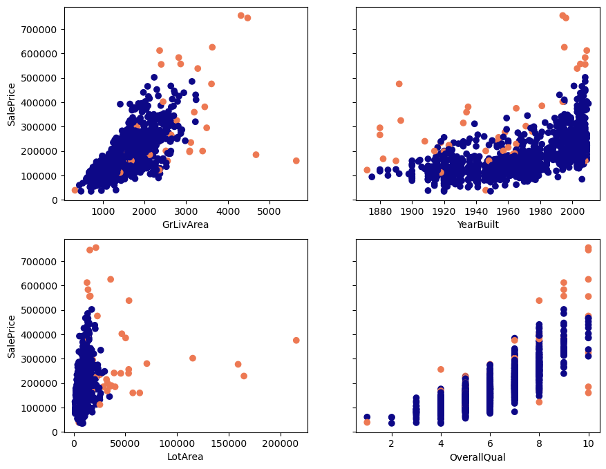
Below, you see scatterplots of the data I will use in this article. It’s housing data from OpenML (Creative Commons license). The plots and data make it easier to explain the detection techniques. I’ll only use four features (GrLivArea, YearBuilt, LotArea, OverallQual) and the target SalePrice. The data contains 1460 observations.
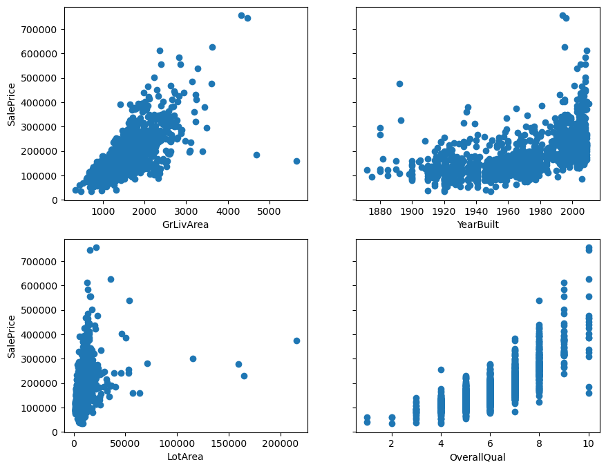
Which points do you expect will be detected as outliers, based on looking at these plots? 🤓
Code to load the data and to plot the outliers:
Detection Methods
Let’s dive in! The three detection methods I will discuss are Cook’s distance, DBSCAN, and Isolation Forest. Feel free to skip the sections you are familiar with.
1. Cook’s Distance
The original article that presented Cook’s distance [1] is titled: Detection of Influential Observation in Linear Regression. That’s exactly what Cook’s distance does: It measures how much influence a data point has on a regression model. The method calculates the Cook’s distance for a data point by measuring how much the fitted values in the model change when you remove the data point.
The higher the Cook’s distance of a data point, the more influence this point has on the determination of the fitted values in the model. If a data point has a high Cook’s distance compared to the other Cook’s distances, it is more likely that the data point is an outlier.
In Python, it’s easy to calculate the Cook’s distance values. After building a regression model you can calculate the distances right away. Below you can see a plot of the Cook’s distance values by Id:
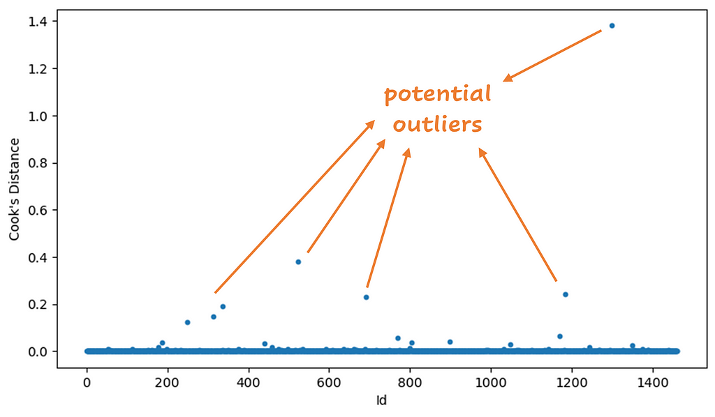
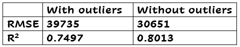
There are different ways to determine which points you want to mark as outlier. Any value higher than 4/n, where n is the sample size (1460 in this example), is interesting to investigate. Another way is to calculate the mean µ of the Cook’s distances, and remove values that are greater than 3*µ. I used the last method to determine the outliers. There were 28 outliers with this method. I retrained the model without them. Below you see the results, good improvement, right? Beware! You have to investigate outliers before removing them! Later more about this.
Outliers according to the Cook’s distance in orange:

Code to calculate the Cook’s distance and to show the outliers:
2. DBSCAN
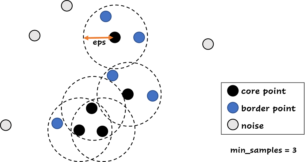
You probably know DBSCAN (Density-Based Spatial Clustering of Applications with Noise) as a clustering technique. Given a dataset, DBSCAN finds core samples of high density and uses these samples to create clusters [2]. You don’t have to specify the number of clusters (as with K-Means), this is a nice advantage of DBSCAN.
With DBSCAN, you have to specify two parameters: the epsilon (eps) and the minimum samples (min_samples). Epsilon is the distance measure and the most important parameter: It is the maximum distance between two samples for one to be considered as in the neighborhood of the other. The minimum samples is the number of samples in a neighborhood for a point to be considered as a core point. This includes the point itself, so if min_samples is equal to 1, every point is a cluster.
DBSCAN can be very useful for detecting outliers. DBSCAN divides the data points in three groups: a group with core data points, these points have at least min_samples in a distance less than eps from them. Than there are the border points, these points have at least one core point in a distance less than eps from them. And the last group contains the points that aren’t core or border points. These points are noise points, or potential outliers. The core and border points receive their cluster number, and the noise points receive the cluster -1.
Before using DBSCAN for outlier detection, it might be necessary to scale your data. I used a StandardScaler in this example, because the data features have very different scales (OverallQual has values from 1–10, YearBuilt values from 1860–2020 and LotArea from 0–250000).
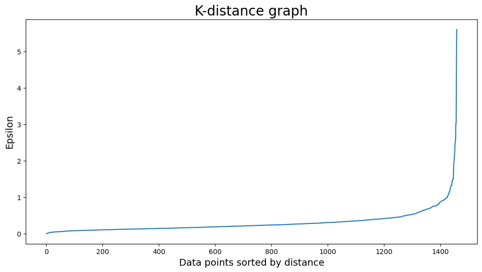
How to find the right values for eps and for min_samples? For min_samples, you can use the rule of thumb D+1, where D is equal to the number of dimensions in the dataset. In this example we will use min_samples = 6. The parameter eps is a bit harder, you can use a K-distance graph to find the correct value. Do you see the elbow? The value of eps is around 1, I used 1.1 for the final run.
Below you see plots of the regular points and the outliers. The orange dots are the outliers according to DBSCAN when we use an epsilon of 1.1 and minimum samples of 6.
Code DBSCAN:
3. Isolation Forest
As anomaly detection model, isolation forests are great. How does it work?
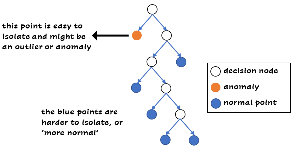
An isolation forest exists of trees, like a normal random forest. In every tree, random features are selected and random split values between the maximum and minimum value of the feature. For every sample, you can calculate the number of splits needed in the tree to isolate this sample. The shorter the average path length to the sample, the more likely that it’s an anomaly (or outlier). This makes sense right? If you need less splits to get to a data point, it’s different from the other data points, because the point is easier to isolate:
You can also apply this technique to categorical data, because of the flexibility of trees.
What about the parameters of an isolation forest? Some of the parameters are the same as those in a normal random forest: you can choose the number of trees (n_estimators), the maximum number of samples for each tree (max_samples) and the number of features for training (max_features). There is one important other parameter: the contamination. You can think of the contamination as the proportion of outliers in the data set. It is used to determine the threshold to decide which points are outliers. If you want the data points and their anomaly scores ranked, you can use the decision_function in scikit learn. And sort the values ascending: the higher the score, the more normal the point.
There is a disadvantage with isolation forests. Edge points that are normal are also easy to isolate. These points have a chance to be classified as outlier, while they are normal. Keep this in mind when using this technique.
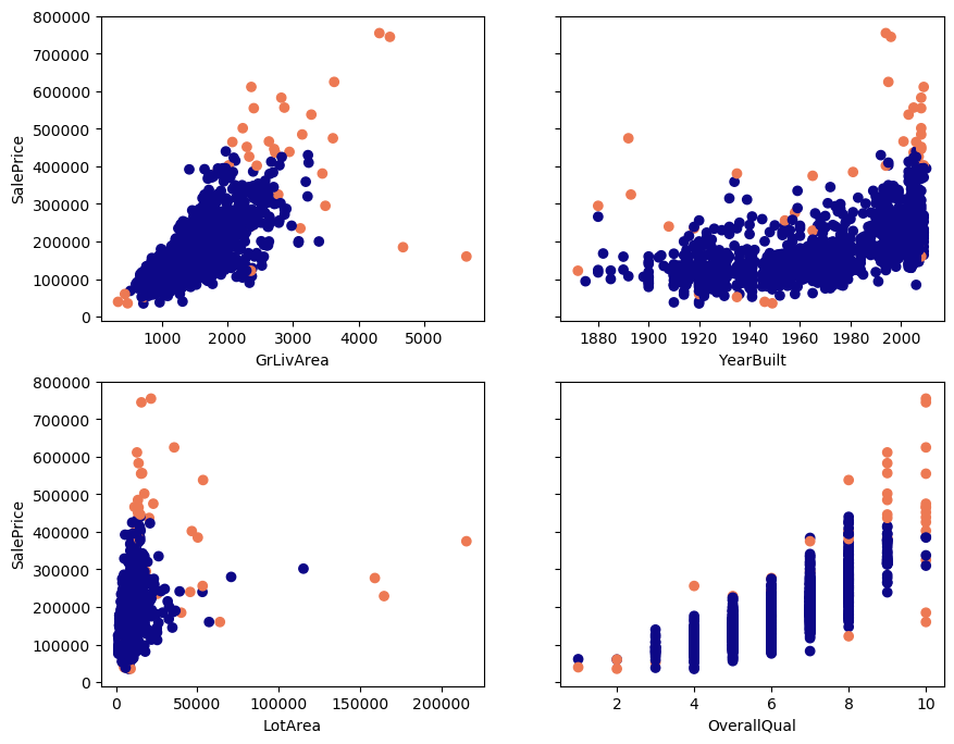
Outliers (in orange) found by Isolation Forest:
Code to find outliers with the Isolation Forest:
Comparison of the techniques
But wait… None of the three outlier detection techniques finds exactly the same outliers as another one! Strange, isn’t it? 19 points are detected by all three techniques, while another 42 points are detected by two or just one technique:
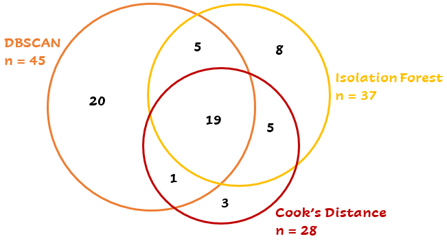
This depends partly on the parameters and the differences between the methods. A short summary: Cook’s distance uses a trained model to calculate the influence of every point, DBSCAN uses the distances between the points and the Isolation Forest calculates the average path length to the points. Depending on the case, you can choose the best technique.
What’s next?
After detecting the outliers, what should you do with them? I hope you don’t just throw them away like they never existed! They came into the dataset so there is a chance it will happen again if you don’t do anything to prevent it.
You can find tips about handling outliers in the article below:
Don’t throw away your outliers!
References
[1] Cook, R. D. (1977). Detection of Influential Observation in Linear Regression. Technometrics, 19(1), 15–18. doi:10.1080/00401706.1977.10489493
[2] Ester, M., H. P. Kriegel, J. Sander, and X. Xu, “A Density-Based Algorithm for Discovering Clusters in Large Spatial Databases with Noise”. In: Proceedings of the 2nd International Conference on Knowledge Discovery and Data Mining, Portland, OR, AAAI Press, pp. 226–231. 1996
Are You Using Feature Distributions to Detect Outliers? was originally published in Towards Data Science on Medium, where people are continuing the conversation by highlighting and responding to this story.
from Towards Data Science - Medium https://ift.tt/si3pAfh
via RiYo Analytics


ليست هناك تعليقات