https://ift.tt/eBKOa9X Implementing logistic regression to predict price elasticity of demand Photo by Artem Beliaikin on Unsplash In...
Implementing logistic regression to predict price elasticity of demand

In this series, we are learning the STP Framework (Segmentation, Targeting, and Marketing), one of the most popular marketing approaches. In the first three posts, we’ve learned to understand our customers using segmentation and divided our customer base into four segments based on their demographics, psychographics, and behavioral characteristics. That covers the first step of the STP Framework.
Our four segments of customers are:
- Standard
- Career-focused
- Fewer-opportunities
- Well-off
In the Targeting step, we define strategies for our customer segments based on the overall attractiveness, strategic direction, market expertise, future potential, etc. Since this falls more into the company strategy under the marketing department, we’ll skip this step in this blog series, and move to the third step, Positioning.
As always, the notebook and the dataset are available in the Deepnote workspace.
Positioning
Positioning is a crucial part of marketing strategy, specially when the firm operates in a highly competitive market. We need to understand how consumers perceive the product offering and how it differs from other competitive offerings. Pricing and discounts play a vital role in shaping customer purchase decisions.
In this post, we’ll employ the logistic regression to understand how the price of a product influences a purchase decision and whether or not we have price elasticity.
But before that, let’s get introduced to the dataset. We will work with a new dataset prepared for this experiment, which leverages the segmentation step that we performed in the previous part.
Data Exploration
We’ll be working with a dataset that represents the customer purchase activities of a retail shop. This dataset is linked with the already familiar customer details dataset that we have already worked with in the earlier three parts of the series (part 1, part 2, and part 3). Every record in this dataset represents a purchase history of a customer.
Here is a detailed description of each attribute:
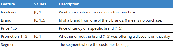
Other calculated attributes:
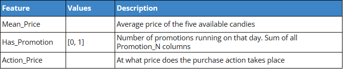
Mean_Price is going to be the primary feature of our experiment in finding the price elasticity. Has_Promotion and Action_Price are secondary features that might help us improve the model. We’ll see.
Let’s start our data exploration with the number of unique customers per segment. We see that the biggest segment is the “fewer-opportunity” segment (38%), and other segments are almost of equal weight (around 20%). That is a well-balanced dataset we are working with.
Each segment also looks quite balanced in terms of the number of actual purchase records (Incidence = 1).
Now, when we look at the average price of each segment, they look very similar. All of them are at around the 2.0 level. But as we narrow our focus and look at the actual purchase price, we can see the “well-off” segment has a higher average price point (2.2), and the “career-focused” customers are at an even higher price point (2.65).
This information is in line with our knowledge acquired in the segmentation part of this blog series. Now let’s move on to the machine learning part where we try to understand the range of price elasticity.
Logistic Regression Model
Logistic regression is a classification algorithm. It estimates the probability of an event occurring, such as loan default prediction. Since the outcome is a probability, it can be either 0 or 1, and for binary classification, a probability less than 0.5 will predict 0 while a probability greater than 0 will predict 1.
In our case, we are not actually going to use the model for binary classification (whether or not a customer make a purchase). Instead, we’ll estimate the price elasticity of the demand and predict how much we can raise the price keeping the market unharmed?
Learn more about logistic regression.
From the model coefficient, it’s evident that there is an inverse relationship between average price and a purchase event. If the average price decreases, the purchase probability will increase.
Now let’s build on this premise.
We see that the price of candy (among all brands) ranges from 1.1 to 2.8. So, keeping some buffer, let’s take the price range from 0.5 to 3.5, increasing 0.01 at a time, and check how the probability of the purchase event changes.
Conclusion
As expected, we observe that as the mean price increases, the chance of purchase decreases.
We shall continue our experiment of price elasticity prediction in the next post and learn how much we can increase the price without breaking the demand.
For more of my content, follow me on medium, and let’s connect on LinkedIn.
Predicting price elasticity of demand with Python (Implementing STP Framework - Part 4) was originally published in Towards Data Science on Medium, where people are continuing the conversation by highlighting and responding to this story.
from Towards Data Science - Medium https://ift.tt/bNSQFnR
via RiYo Analytics


No comments