https://ift.tt/9pSaELA Nature-inspired algorithm explained with simple code and animation Photo by Sebastian Pena Lambarri on Unsplash ...
Nature-inspired algorithm explained with simple code and animation

In this article, we explore the theoretical aspects of the nature-inspired optimisation algorithm, Particle Swarm Optimisation, and then apply the algorithm to a simple example in Python, representing it in an animated gif so that we can see how it works.
If you are training a deep learning model with a stochastic gradient descent with backpropagation and cannot escape from the local minima, this article may help you to find an alternative approach to resolve the problem.
A swarm is a collection of agents or organisms; swarm intelligence can be defined as the social behaviours of a swarm in which autonomous individuals interact with each other in a decentralised and self-organised manner. The interaction of individuals improves the empirical knowledge about the environment and brings the swarm to the optimal state.
We can observe such intelligence in nature. For example, ants are known to find the shortest path from their colony to a food source. In the beginning, individuals explore various directions from and to the destination. When a favourable route is found, ants mark the path with pheromones which are chemical substances ants deposit on the ground. As more ants take the same trail, the pheromones intensify, attracting more ants. Consequently, the majority of ants follow and converge to the shortest path.

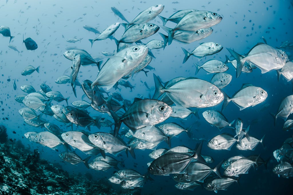
There are some nature-inspired algorithms that mimic swarm intelligence. Ant Colony Optimisation (ACO) is derived from ants. Artificial Bee Colony (ABC) is inspired by honeybees swarming around their hives. This article is about Particle Swarm Optimisation (PSO) which is hinted at by bird flocking and fish schooling.
PSO was initially introduced by James Kennedy and Russell Eberhart in 1995. [1] [2] They hypothesised that the social sharing of the information would offer advantages to the swarm. Rather than competing for food, individual members of the fish school can profit from other members’ discoveries and experiences whenever the resource is distributed beyond prediction. The key word is “social interaction”. Social behaviour increases the capability of an individual to adapt; as a result, intelligence emerges in the swarm. The adaptability of individuals and collective intelligence are related to each other.
The algorithm of PSO is simple. Particles are a number of simple entities in a search space. We create a population of particles and measure their individual fitness with an objective function of the problem. Particles are then moved from their current to the next position based on their personal best location, and on the swarm’s best location so far. By iterating the moves the swarm gradually reaches an optimal point of the objective function over generations.
Some notations:
Number of particles         : i
Number of dimensions        : n
Fitness function            : f(x_i)
Particles                   : x_i = (x_i1, x_i2, ..., x_in)
Current velocity            : v_i = (v_i1, v_i2, ..., v_in)
Individual particle's best  : p_i = (p_i1, p_i2, ..., p_in)
Global particles' best      : p_g = (p_g1, p_g2, ..., p_gn)
Inertia component           : w * v_i(t)
Cognitive component         : c_1 * r_1 * (p_i - x_i(t))
Social component            : c_2 * r_2 * (g_i - x_i(t))
Velocity adjustment         : v_i(t+1) <- Inertia+Cognitive+Social
Position adjustment         : x_i(t+1) <- x_i(t)+v_i(t+1)
The velocity adjustment is influenced by 3 factors: the previous velocity (Inertia component), the individual particle’s best position (Cognitive component) and the swarm’s best positions (Social component). The velocity is a speed of a moving particle to a given direction. The particle’s movement is affected by these weights in each direction. The coefficient w is called inertia weight which is a force to keep the particle moving in the same direction as the previous generation. c1 and c2 are constant acceleration values where c1=c2 is applied in the original algorithm by [1]. r1 and r2 denote hyper parameters and they cause some random perturbations. The higher value of these parameter values results in a more responsive movement of the particles. We also assume that the fitness function is for the minimisation problem in our case. Therefore the individual particle’s best position p_i is over-written by x_i when f(x_i) < f(p_i).
PSO Algorithm is as follows:
1. Initialise the particle population array x_i
2. Loop
3. For each particle, calculate the fitness using the
   fitness function f(x_i)
4. Compare the current fitness value with its best p_i.
   Replace the best with the current value x_i
   if it is better than the best.
5. Check the swarm’s best particle from individual particle’s best
   and assign the best array to the global best p_g.
6. Calculate the velocity v_i(t+1) and update the position of
   the particles to x_i(t+1)
7. If a criterion is met, exit the loop.
8. End loop
Let’s translate the algorithm into Python code. In order to visualise the particles’ movement, we can simplify the particles’ dimensions to two, x and y. The scripts are written procedurally.
1. Import libraries
2. Define fitness function
We use the function: f(x,y)=(x-2y+3)^2+(2x+y-8)^2. The global minimum of this function is 0. All particles should move from random points towards the optimal position of x and y coordinates, where the value becomes near 0.
3. Update velocity
We apply the random values for r1,r2 and w. c1 and c2 are given smaller values at 0.1. The inertia value can be scheduled; starting from 0.9 and gradually reducing to 0.4. In our case, we generate the normal distribution with min 0.5 and max 1 and randomly select a value at each generation, following the experiments by [3].
4. Update position
As described in the algorithm, the new position is a sum of the current position and velocity.
5. PSO's main function
Firstly, we initialise the particles, their best position, velocity and fitness value. We also set the global best position based on the particles’ initial position. Then we loop from one generation to another. The algorithm should stop when it reaches the max number of generations or a success criterion. In our case, it is when the average fitness value surpasses a specific value.
6. Set parameter values and run the algorithm
population = 100
dimension = 2
position_min = -100.0
position_max = 100.0
generation = 400
fitness_criterion = 10e-4
We created 100 particles, of which positions were randomly placed at x and y coordinates, ranging between -100 and 100. As the function takes x and y, the particle’s position is 2-dimensional. The success criterion is 0.001 or lower. The programme should stop before the 400th generation if the criterion is met.
By running the algorithm with the above configurations, we obtained the following outcome:
Global Best Position:  [2.60008033 2.799968  ]
Best Fitness Value:  3.7383573411040855e-08
Average Particle Best Fitness Value:  0.0009671024787191154
Number of Generations:  68
Because of its stochastic nature, the result changes every time you run the programme. It took 68 generations to achieve the success criterion. The best particle reached the positions x≈2.6 and y≈2.8, where the fitness function returns the global minimum.
Rather than having the results in text, it would be much more insightful if we could visualise the particles’ movements.
7. Matplotlib plot and animation
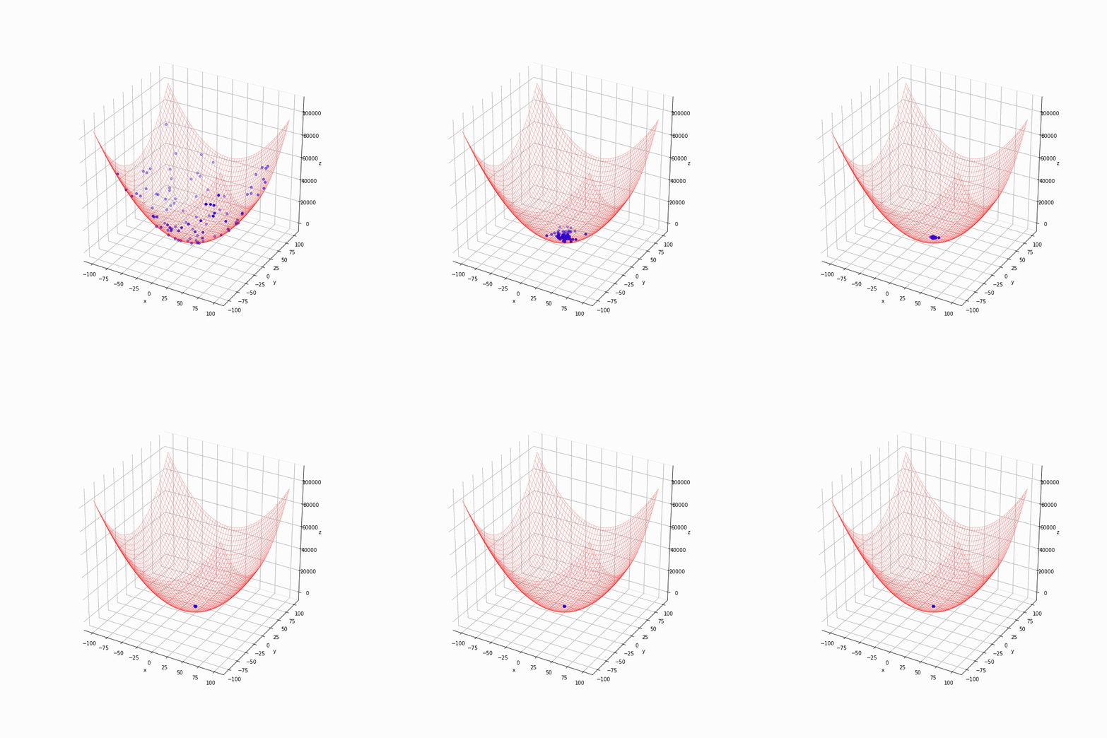
Drawing a wireframe of the functions helps to see where is the global minimum. The image should be captured for each generation. Below is the output for the same example.

In the first generation, the particles are scattered. They quickly move towards the bottom of the grid, and it looks like the algorithm is working as expected. We could do some more experiments by changing the fitness functions and hyper-parameters like the inertia weight w and cognitive and social coefficients (c1 and c2) to optimise the algorithm.
Swarm intelligence like PSO is a class of metaheuristics that is believed to find a near-optimal solution for complex optimisation problems with a reasonable computational time. It is especially useful if we apply the algorithm to train a neural network. The benefit is twofold: global search and parallelisation.
We can translate each particle to be an n-dimensional array that represents the weights between neurons. As we saw in the animated gif, each particle makes a movement in a different direction. Unlike the backpropagation learning algorithm that searches the optimum point locally, PSO makes it possible to explore many different sets of weight parameters simultaneously, thus helping to avoid the path to the local minima. Furthermore, the fitness function is independent of a network topology; the computation to evaluate each particle’s fitness can be parallelised.
This article explored the particle swarm optimisation algorithm with a simple code to understand the mechanics. If you find PSO application to ML interesting, I highly recommend checking out the following article on the integration of machine learning into various meta-heuristics.
Reference:
[1] J. Kennedy and R. Eberhart, “Particle swarm optimization,” Proceedings of ICNN’95 — International Conference on Neural Networks.
[2] Poli, R., Kennedy, J. & Blackwell, T. Particle swarm optimization. Swarm Intell 1, 33–57 (2007). https://doi.org/10.1007/s11721-007-0002-0
[3] R. Eberhart and Yuhui Shi, “Particle swarm optimization: Developments, applications and resources,” Proceedings of the 2001 Congress on Evolutionary Computation (IEEE Cat. №01TH8546), Aug. 2002.
Swarm Intelligence: Coding and Visualising Particle Swarm Optimisation in Python was originally published in Towards Data Science on Medium, where people are continuing the conversation by highlighting and responding to this story.
from Towards Data Science - Medium https://ift.tt/LkKaPiZ
via RiYo Analytics

No comments