https://ift.tt/RkLbtqT Learn how to visualize text data to convey your story Free for Use Photo from Pexels Introduction There are va...
Learn how to visualize text data to convey your story

Introduction
There are various definitions of Natural Language Processing (NLP) but the one I often quote is the following:
NLP strives to build machines that understand and respond to text or voice data — and respond with text or speech of their own — in much the same way humans do. [1]
The NLP market is growing fast because of the increasing amounts of text data that are being generated in numerous applications, platforms and agencies. Thus, it is crucial to knowing how to convey meaningful and interesting stories from text data. For that, you need visualization. In this post, let us learn on how to get started on visualizing text data. More advanced methods of pre-processing and visualizing text data will be introduced in another post!
Visualizing Distributions of Basic Summary Statistics of Text
The concept of “summary statistics” for tabular data applies to text data in a similar fashion. Summary statistics help us characterize data. In the context of text data, such statistics would be things like number of words that make up each text and how the distribution of that statistic looks like across the entire corpus. For looking at distributions, we can use visualizations including the kernel density estimate (KDE) plot and histogram etc. but for the purpose of just introducing what statistic could be considered for visualization, the .hist( ) function is used in all the code snippets.
Say we have a review dataset which contains a variable named “description” with text descriptions in it.
[1] length of each text
reviews[‘description’].str.len().hist()
[2] Word count in each text
# .str.split( ) returns a list of words split by the specified delimiter
# .map(lambda x: len(x)) applied on .str.split( ) will return the number of split words in each text
reviews[‘description’].str.split().map(lambda x: len(x)).hist()
Another way to do it:
reviews[‘description’].apply(lambda x: len(str(x).split())).hist()
[3] Unique word count in each text
reviews[‘description’].apply(lambda x: len(set(str(x).split()))).hist()
[4] Mean word length in each text
reviews[‘description’].str.split().apply(lambda x : [len(i) for i in x]).map(lambda x: np.mean(x)).hist()
Another way to do it:
reviews[‘description’].apply(lambda x: np.mean([len(w) for w in str(x).split()])).hist()
[5] Median word length in each text (Distribution)
reviews[‘description’].apply(lambda x: np.median([len(w) for w in str(x).split()])).hist()
[6] Stop word count
Stopwords in the NLP context refers to a set of words that frequently appear in the corpus but do not add much meaning to understanding various aspects of the text including sentiment and polarity. Examples are pronouns (e.g. he, she) and articles (e.g. the).
There are mainly two ways to retrieve stopwords. One way is to use the NLTK package and the other is to use the wordcloud package instead. Here, I use the wordcloud package as it already has a full set of English stopwords predefined in a sub-module called “STOPWORDS”.
from wordcloud import STOPWORDS
### Other way to retrieve stopwords
# import nltk
# nltk.download(‘stopwords’)
# stopwords =set(stopwords.words(‘english’))
reviews[‘description’].apply(lambda x: len([w for w in str(x).lower().split() if w in STOPWORDS])).hist()
[7] Character Count
reviews[‘description’].apply(lambda x: len(str(x))).hist()
[8] Punctuation Count
reviews[‘description’].apply(lambda x: len([c for c in str(x) if c in string.punctuation])).hist()
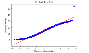
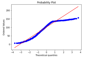
Bonus: Checking Normality
For new statistic variables (e.g. mean word length) created, you may want to c heck whether they meet certain conditions as certain models or regression algorithms require variables to fall under certain distributions, for example. One such check would be checking if the distribution of a variable is close enough to a normal distribution by looking at the probability plot.
from scipy import stats
import statsmodels.api as sm
stats.probplot(reviews['char_length'], plot=plt)
Visualizing Top N-Grams
What is an n-gram? According to Stanford’s Speech and Language Processing class material, an “n-gram is a sequence n-gram of n words in a sentence of text.” [2]
For instance, bigrams (n-gram with n=2) of the sentence “I am cool” would be:
[ (‘I’, ‘am”), (‘am’, ‘cool’)]
To visualize the most frequently appearing top N-Grams, we need to first represent our vocabulary into some numeric matrix form. To do this, we use the Countvectorizer. According to Python’s scikit-learn package documentation, “Countvectorizer is a method that converts a collection of text documents to a matrix of token counts.” [3]
The following function first vectorizes text into some appropriate matrix form that contains the counts of tokens (here n-grams). Note that the argument stop_words can be specified to omit the stopwords from the specified language when doing the counts.
def ngrams_top(corpus, ngram_range, n=None):
### What this function does: List the top n words in a vocabulary according to occurrence in a text corpus.
vec = CountVectorizer(stop_words = ‘english’, ngram_range=ngram_range).fit(corpus)
bag_of_words = vec.transform(corpus)
sum_words = bag_of_words.sum(axis=0)
words_freq = [(word, sum_words[0, idx]) for word, idx in vec.vocabulary_.items()]
words_freq =sorted(words_freq, key = lambda x: x[1], reverse=True)
total_list=words_freq[:n]
df = pd.DataFrame(total_list, columns=[‘text’,’count’])
return df
The following function specified the ngram_range to be (1,1), so we are only interested in unigrams which are basically just individual words. n=10 here means we are interested in looking at the top 10 unigrams in the corpus of descriptions.
unigram_df = ngrams_top(reviews[‘description’], (1,1), n=10)
We then can visualize this into a horizontal bar plot using seaborn.
# seaborn barplot
sns.barplot(x=’count’, y=’text’) #horizontal barplot
If you want to use a slightly fancier and interactive form of visualization, I recommend plotly express which has very simple syntax but enables you to create interactive visualizations in a few lines of code.
# fancier interactive plot using plotly express
import plotly.express as px
fig = px.bar(unigram_df, x='unigram', y='count', title=’Counts of top unigrams', template='plotly_white', labels={'ngram;: ‘Unigram’, ‘count’: ‘Count’})
fig.show()
More advanced methods of pre-processing and visualizing text data will be introduced in another post!
About the Author
Data Scientist. Incoming PhD student in Informatics at UC Irvine.
Former research area specialist at the Criminal Justice Administrative Records System (CJARS) economics lab at the University of Michigan, working on statistical report generation, automated data quality review, building data pipelines and data standardization & harmonization. Former Data Science Intern at Spotify. Inc. (NYC).
He loves sports, working-out, cooking good Asian food, watching kdramas and making / performing music and most importantly worshiping Jesus Christ, our Lord. Checkout his website!
References
[1] What is Natural Language Processing?, IBM Cloud, https://realpython.com/python-assert-statement/
[2] D. Jurafsky & J. H. Martin. Speech and Language Processing (Last Updated December, 2021). https://web.stanford.edu/~jurafsky/slp3/3.pdf
[3] Scikit Learn documentation. https://scikit-learn.org/stable/modules/generated/sklearn.feature_extraction.text.CountVectorizer.html
Getting Started with Text/NLP Visualization was originally published in Towards Data Science on Medium, where people are continuing the conversation by highlighting and responding to this story.
from Towards Data Science - Medium https://ift.tt/Doe2kJw
via RiYo Analytics


No comments