https://ift.tt/AnxMNRe Analytical and numerical perspectives of the problem of Continuous Blackjack Photo by Erik Mclean on Unsplash ...
Analytical and numerical perspectives of the problem of Continuous Blackjack

Introduction
This is the first of several posts where we will analyze the problem of playing continuous blackjack. In particular, we want to extend the work of Henry Charlesworth and Mu Zhao to other distributions. In this first post, we will reproduce the existing results and propose a way to extend them to other distributions. Then, we will analyze the case of the uniform distribution and show some interesting plots.
Problem Statement
Consider the continuous version of the blackjack game, which has the following rules:
- Each player i starts with an empty stack S_i=[]. The value of this stack is defined as V_i=∑|S_i|S_ji.
- A dealer draws random values from a distribution P(x).
- The players play the game in turns. The turn of every player starts by receiving a number from the dealer and adding to its stack S_i. Then, the player has two options:
- Decide to stop playing and finish the game with its current stack. Then the player’s turns end and it is the turn of the next player.
- Get another number, add it to its stack, and go back to step 3. The player can do that all the times they want while V<1. If V>1 the player automatically loses and the turn of the next player starts.
- The player with the highest value V wins the game.
The question is, what’s the best strategy to win this game?
Preliminaries
To start let us define F(t;a,b) to be the probability of landing in the interval R=(a,b), given that we are actually at t and we are going to keep playing if t<a. This probability can be split into two parts, (1) the probability that we land on R in the next turn, and (2) the probability that we don’t land on R on the next turn but in one of the following ones.
In mathematical terms this is

Uniform distribution
In the particular case of P=U[0,1]

And differentiating with respect to t on both sides we get

The constant K can be obtained using F(a;a,b)=b−a, so K=(b−a)e^a.

Notice how the equation doesn’t depend on the particular value of a, b, and t but on the distances between them. Thus, one can define the value W=b−a as the width of the range, and D=t−a as the distance from the current location to the lower bound. Then, the equation can be written as

Strategies
In this section, we will analyze how to use the results derived in the last section to find the optimal strategy in different scenarios.
1 vs 1
Let’s start with the simplest case: you’re playing against only one other person. The first player gets a point if the second player busts. If the first player’s score is s, then the second player has a probability of 1−F(0;s,1) to bust, this means that our probability to win if we stay at s is 1−F(0;s,1). Of course, if we could choose our s we would choose s=1, but since this is a random process we can’t choose s. The only thing we can choose is at which α we stop drawing numbers. This α is defined by the following point: where the probability of winning given that we stick at α is the same as the probability that we win given that we draw one more number.
Specific case: uniform distribution
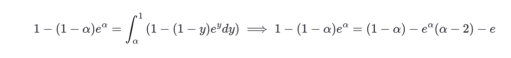
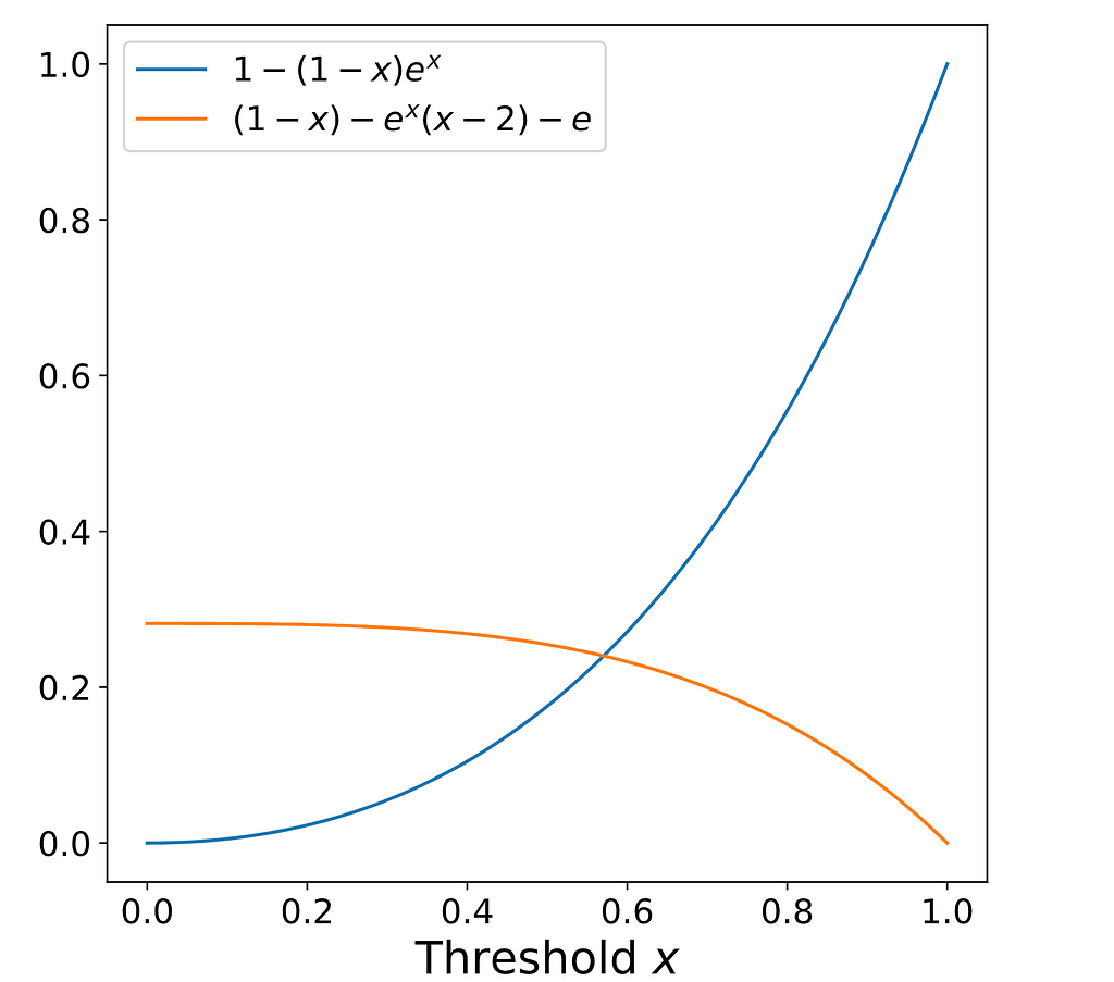
For this section let’s assume that P=U[0,1] and that all the players start at x=0. In this case, the condition described by the above reasoning is written as

Notice that the left side is increasing, while the right side is decreasing.
Simulation results
Before moving to theoretical results, let’s try to find the optimal threshold via simulations. To do so, we will try each possible threshold and simulate 50000 games. Then we will check the probability of the first player winning as a function of the chosen threshold. The results are plotted in the following plot:
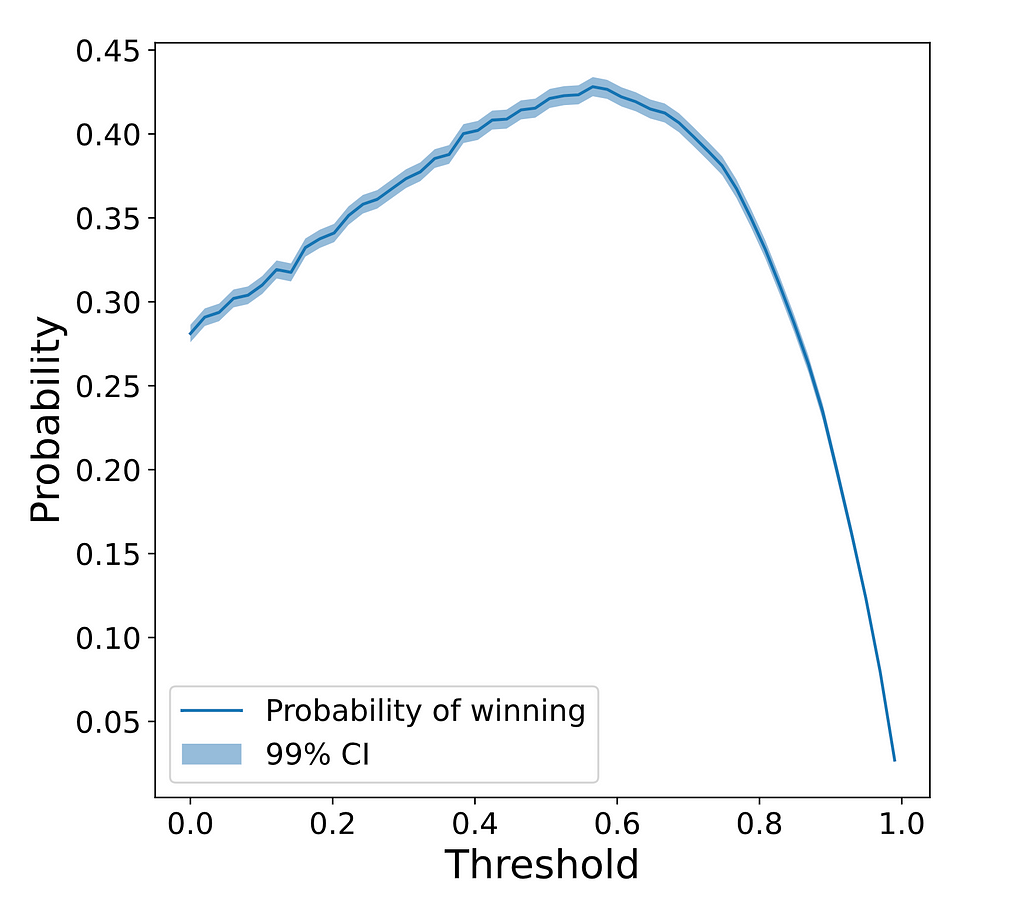
As you can see, the maximum winning probability is achieved around t∗=0.6, more specifically is t∗=(0.565±0.035). To compute the optimal threshold and its deviation we have run a Monte-Carlo simulation. This is, we have generated 1000 samples of the threshold-vs-probability curve using the expected winning probability and its 99% confidence interval. Then, we have computed the optimal threshold for each of these samples, and from this set of optimal thresholds, we have computed the average and standard deviation.
Knowing the range where the optimal value lies, let’s repeat the above simulations but only with thresholds between 0.5 and 0.65. Using this smaller range we get the optimal threshold t∗=(0.568±0.021). Finally, the expected winning probability at the optimal threshold is p_win(t∗)=(0.4278±0.0011). Let’s see now if the analytical results are compatible with the simulations.
Analytical results
Using the results from section Uniform Distribution and P=U[0,1], the equation for the optimal α is
This is a non-linear equation without a closed form, but it can be solved approximately using numerical methods, and the solution is α∗≈0.5706. This means that when the accumulated value of our stack gets bigger than 0.5706 we should end our turn. This result is compatible with the range we found in our simulations.
Conclusions
In this first post, we have derived the generic equation for the probability of falling in a range (a,b) given that we’re currently at t. We have also derived the condition that the optimal thresholds have to fulfill. Finally, we have studied the particular case of the uniform distribution — both numerically and analytically — and studied its properties.
In the following posts, we will study how all these results change when the distribution P changes. We will also study the case where we play against N players instead of only one.
This story was originally published here.
Continuous Blackjack (i): Introduction and First Results was originally published in Towards Data Science on Medium, where people are continuing the conversation by highlighting and responding to this story.
from Towards Data Science - Medium https://ift.tt/E7BMc3j
via RiYo Analytics


No comments