https://ift.tt/3o5A73V We review the difference between marketing mix modelling (MMM) vs multi-touch attribution (MTA) and then we go on ...
We review the difference between marketing mix modelling (MMM) vs multi-touch attribution (MTA) and then we go on to build a simple MMM model in R

TLDR
In a previous article, we discussed how to clean and prep messy marketing data using R prior to analysis or modelling. Here, we’ll dive into marketing mix modelling. Specifically, we will look at:
- An overview of marketing mix modelling
- The difference between marketing mix modelling vs multi-touch attribution models. Both may seem similar but are applied in very different scenarios. They can also be used together!
- Building a basic marketing mix model using R
- Defining Adstock
- Interpreting the results of the marketing mix model
- Making predictions and recommendations
Just like in the previous article, I’ve written this in an easy-to-follow manner using a very basic example. The R code has been extensively commented and presented step-by-step to help new R users try this technique out.
What is marketing mix modelling and why is it useful
Marketing mix modelling (MMM) is an econometric method to estimate the impact of advertising channels on key conversion outcomes (e.g. sales, customer activation, leads, etc). A brand may use different types of marketing tactics to increase awareness about their products and drive sales. For example:
- Using email marketing to entice new customers with a discount code for first-time purchases
- Through paid media campaigns such as pay-per-click or digital display advertising on Youtube
- Via social media like Facebook
- Or through offline traditional OOH (out-of-home) media such as TV, print or radio
This is why it is called the marketing “mix” because there is more than one channel running marketing campaigns at any given time. Marketing budgets will vary across channels and each channel’s ability to drive awareness and sales will differ from one another.
For example: as a channel, primetime ads on TV would most likely be significantly expensive compared to say, display advertising. And whilst social media platforms are great for raising awareness and developing a community, it is not always considered a converting channel, unlike the immediacy of pay-per-click (PPC) where sales can happen on the same day users click on PPC ads. Obviously, these examples vary depending on the brand, industry or product being marketed.
By performing marketing mix modelling, brands can determine how effective a particular marketing activity is on critical outcomes like sales. It can be used to estimate the return of investment for a given channel and even be used as a planning tool to optimise spends and predict / benchmark future performance.
What is the difference between marketing mix modelling (MMM) and multi-touch attribution (MTA)
These modelling techniques sound similar but they are applied in different scenarios.
Marketing Mix Modelling
Explaining this as simply as I can: marketing mix modelling datasets typically include predictors such as spends for each channel and outcome variables like sales or revenue for the given period. We are trying to model the relationship between the spends on each channel against the outcome we care about, in this case sales (or total enquiries, whichever is a key conversion KPI for the brand). In doing so, we uncover the impact each channel has had on sales and we can use this relationship to predict future sales, given spend.
At the risk of over-simplifying: it helps to answer “spend x, get y” type of questions. It can be used to estimate diminishing returns, understand ROI and applied as part of budget planning.
So it is not surprising to see that regression methods like multiple regression being commonly applied in marketing mix modelling.
It is also worth noting that it is difficult to measure performance of offline traditional OOH media like TV, radio and print (unlike online advertising where we have access to metrics like clicks, clickthrough rate, impressions, etc). So spend is used in this case.
Multi-touch Attribution Modelling
In multi-touch attribution, we acknowledge that the customer journey is complex and customers may encounter more than one (or even all) of our marketing channel activities in their journey.
A customer’s path to purchase may have started with seeing a display ad whilst online → got exposed to a social media campaign → later performed a keyword search in Google → and then clicked on a PPC ad before landing on the website and finally completing their purchase.
Unlike MMM where we tend to look at a top-level view of spends, in multi-touch attribution, we care about these granular touchpoints because they all play a part in contributing towards the final sale.
Instead of spends, we assign weighting to these channels based on their touchpoints to determine each channel’s contribution / involvement towards the sale.
Weighting can differ based on how we value each touchpoint. There are several attribution models that can be used to determine the weighting. The more common ones being:
Last click attribution: this assigns 100% weighting to the last channel that was clicked on. So in the above example, PPC would get all the credit. None of the channels before that will be given any credit. This is the default model used in most analytics platforms. This is the easiest weighting to explain because all it says is “this channel is the last one the user encountered before making the purchase, therefore it is the most important because it was the one that drove the final decision.” Google Analytics have used this method for years until recently when data driven attribution was made widely available in Google Analytics 4.
First click attribution: this is the opposite to last click attribution. Here, we assign 100% weighting to the first channel. Using the example above, this would be the display ad. The argument for this method usually goes along the lines of “had display not been the first channel, the subsequent touchpoints would not have occurred anyway, so the first channel is the most important.”
The problem with first and last click is that they ignore the contributions that other channels have played. They are too simplistic.
Then we have models like:
Time-decay: weighting is distributed based on the recency of each channel prior to conversion. The most weighting will be given to the last channel prior to conversion (PPC). The least weighting is assigned to the first channel.
Position-based: the first and last channels each receive 40% of the weighting, with the remainder 20% distributed equally to the middle channels.
Data-driven attribution (DDA): This is perhaps the best method (compared to first, last, time-decay and position-based) because instead of using predetermined rules to assign weighting, weighting is assigned objectively by an algorithm based on the probability of conversion, given the touchpoints. Methods like Markov Chain, game-theory approaches using Shapley values used in media platforms like Google Search Ads 360, and even ensemble methods like Random Forest can be used in DDA.
In most analytics platforms like Google Analytics, applying these models for multi-touch attribution is as simple as clicking and selecting the one you want and using it in your reports.
However note that for multi-touch attribution, the channels need to be able to report on metrics like clicks, clickthrough rates, impressions and so on, so that touchpoints and their sequences can be measured effectively. This means multi-touch attribution is highly suited for digital channels. It is almost impossible to measure metrics like “clicks” on radio.
Can we use both together?
Yes MMM and MTA can be used to complement each other. MMM can be used for a topline view of the effectiveness of spends across both online and offline marketing activities, and then MTA can be applied to drill-down specifically into online channels for deeper insights.
Building a basic marketing mix model using R
The scope of this article is to provide a simple example for marketing mix modelling in R.
👉 Important! You will need to make sure your marketing dataset is clean with channel spends per period (ideally weekly) and sales for each given week. For a guide on how to clean and prep your marketing data prior to performing modelling in R, look at my previous article here.
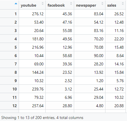
In this example, we will use the sample marketing dataset already available in the datarium package in R. Install it first then let’s load it and take a look:
This is a dataframe of 200 observations (rows) with 4 variables (Youtube, Facebook, Newspaper and Sales), all numeric, and in their thousands. The spends are in £s and sales is taken to be no. of units sold. For the purpose of this exercise let’s assume these are marketing spends across Facebook, Youtube and Newspaper for the past 200 weeks.
Checking correlation
Using the chart.Correlation() function from the PerformanceAnalytics package, let’s visualise the correlation between variables in a nice chart:
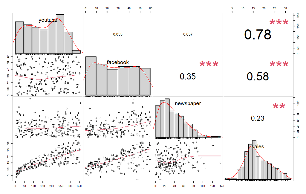
Youtube has a positive relationship with sales — the significance is high and the relationship is strong (0.78). Facebook too has a positive relationship with sales, this is significant but the relationship is moderate (0.58). Newspaper, has a positive relationship with sales though this is quite small (0.23).
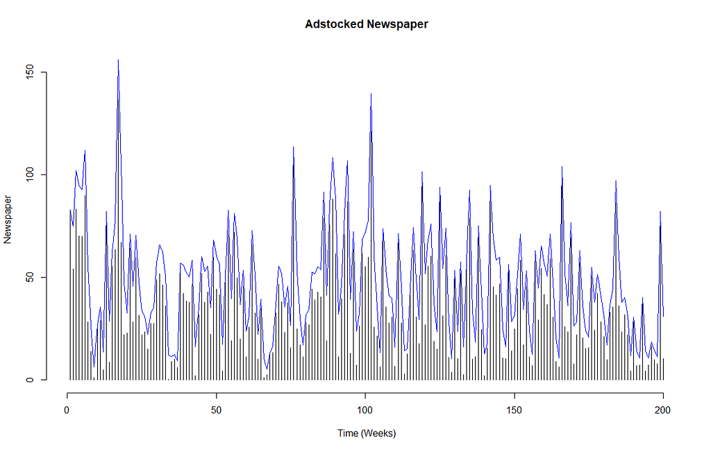
Defining Adstock
In marketing mix modelling, we estimate that the effectiveness of an ad becomes less impactful over time. Adstock theory (Broadbent, 1979) assumes that awareness generated of the product being advertised is highest when the ad was recently viewed. Awareness eventually declines when ad exposure decreases.
Akin to the time-decay multi-touch attribution discussed earlier, adstock is expressed as a decay model, its value is between 0 and 1, with 0 denoting least awareness and 1 denoting 100% awareness. Note that typical adstock transformations assumes an infinite decay and Gabriel Mohanna has articulately argued why this is not always realistic in his post here.
To calculate adstock for the channel, you will need the adstock rate. Most MMM modelling done agency-side will have access to adstock benchmarks which can simply be applied. Impactful creative ads on TV are more memorable and therefore will have a higher adstock rate (e.g. 0.8) compared to online PPC ads (e.g. 0.1 or even 0!) which are usually just text and static in nature.
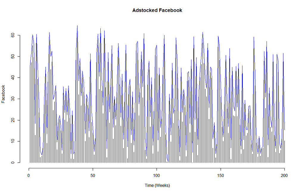
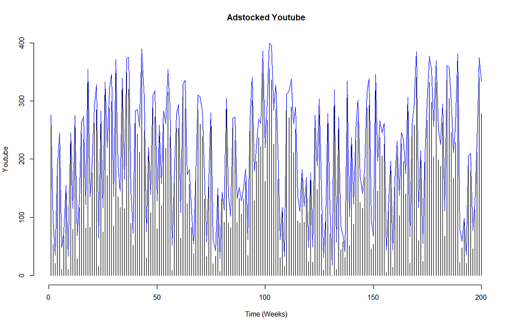
In our example dataset of Youtube, Facebook and Newspaper, we will assume that the Facebook activities are usually simple text posts, the ad on youtube is an animated display banner and the newspaper one is a colouful half-page creative takeover. So Facebook will have the lowest adstock rate (0.1), and the newspaper takeover we will assume to have an adstock rate of 0.25.
Applying Gabriel’s recommendation for adstock transformations, we get the below.
👉Tip: Don’t forget to unload dyplr and tidyr so that they don’t mess with the filter() function below. Alternatively, clearly specify stats::filter() so that it avoids the of the dplyr version. In dplyr::filter(), x is required as a tibble / dataframe.
Building the marketing mix model using multiple regression, checking for multicollinearity and heteroskedasticity
With sales taken to be the dependent variable, we can now build an MMM model using multiple regression with the adstocked values for Youtube, Facebook and Newspaper.
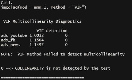
We will fit this into the lm() function. We then apply VIFs (variance inflation factors) using the imcdiag() function from the mctest package to check for multicollinearity and finally we perform a test to check for heteroskedasticity.
The problem with multicollinearity and heteroskedasticity
- 👎Multicollinearity is problematic, especially in regression because it creates a lot of variance in the coefficient estimates, and they become very sensitive to small changes in the model, making the model unstable.
- 👎Heteroskedasticity is also problematic, especially in linear regression because this regression assumes that the random variables from the model have equal variance around the best fitting line — in other words, there should be no heteroskedasticity in the residuals. There should not be any obvious patterns in the variance of residuals against the fitted values of the dependent variable.
- 👎The presence of heteroskedasticity is a flag that the estimators cannot be trusted. The model may be generating inaccurate t-statistics and p-values and can lead to very weird predictions.
In short, the presence of multicollinearity and heteroskedasticity can make our model inaccurate and unusable.
No multicollinearity was detected in the VIF method applied earlier — great🤗!
Heteroskedasticity can be checked by “eye-balling” 👀 the plots :
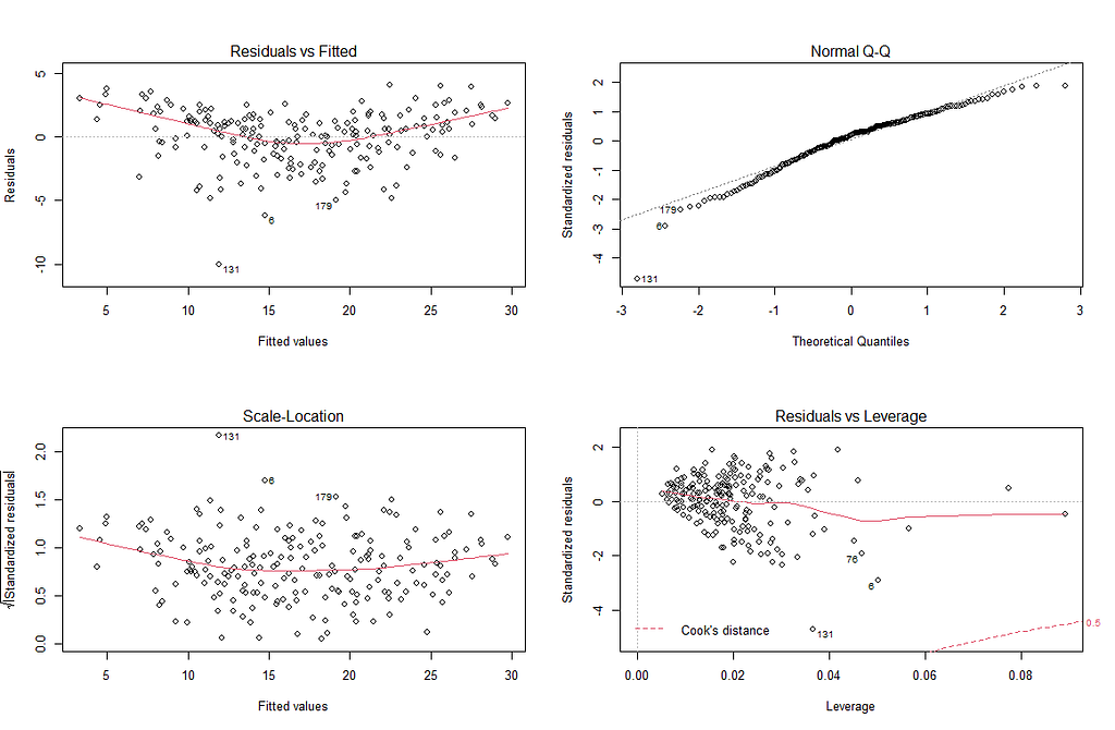
We are most interested in the two graphs on the left. If there was totally no heteroskedasticity, the red line would be completely flat and there should be random and equal distribution points across the x axis. In our Residuals and Fitted plot, if you look closely, there is a dotted line at 0, indicating residual value = 0. Our red line is slightly curved, but does not deviate too heavily from the dotted line. There also does not seem to be an obvious pattern in the residuals. This is good.
The same can be said for the Scale-Location plot, we want the red line to be as flat as possible, with no obvious patterns in the scatterplot points. This seems to be the case.
A more objective method would be to use the Breusch Pagan test using bptest() from the lmtest package and ncvtest() from the car package. Both tests check for heteroskedasticity.
H₀ indicates that the variance in the model is homoskedastic.
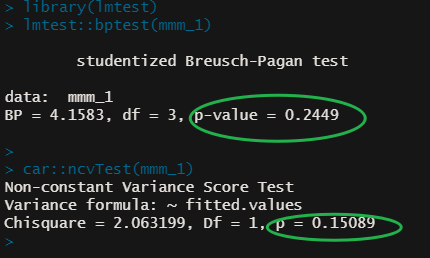
As our p-values from the Breusch Pagan and NCV tests returned values above the significance level of 0.05, we cannot reject the null hypothesis (yay!) 🙌. Hence, we can say that there are no major issues with heteroskedasticity in our model:
Interpreting the summary results from our first model
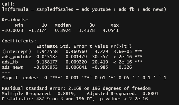
Let’s interpret the summary results of the model:
Observing the coefficient estimates, recall that figures are in their 1000s — yes, I had to remind myself too! 🤦♂ (Channel budgets are in £s and sales is taken to be no. of units sold)
- For every £1000 spent on Youtube, we can expect sales to increase by 45 (0.045*1000) units. For every £1000 spent on Facebook, we can expect sales to increase by 188 (0.188 * 1000) units. For every £1000 spent on Newspapers, we can expect sales to decrease by 6 (0.006 * 1000) units though this is not significant.
- The t-statistics indicate whether we can be confident with the relationship between our features (the channels) and the dependent variable (sales). The high (>1.96) t-statistic for Youtube and Facebook as well as their statistically significant p-values means we can have confidence in the precision of their coefficients. Not so much for Newspapers — but this somewhat makes sense because it is very hard to accurately attribute sales from Newspaper ads (unless a special url or a QR code is included in the creative which can help yield better data collection).
- The R² indicates the goodness of fit, i.e. how well the model fits the data. An R² of 0.88 indicates that the model can be explained by 88% of the data.
Not bad! 😸 Let’s see if we can make this better in the next iteration below.
Including trend and seasonality into the model
We can add trend and seasonality as additional features to the model.
Note that our data is weekly therefore frequency is set to 52 (though this will be tricky on leap years). We also require a minimum of 2 periods (52 x 2 = 104 weeks), our data has observations from the past 200 weeks so this should be sufficient.
To add a basic linear trend of sales to lm(), we could use seq_along() which produces a vector of sequential integers:
basic_trend <- seq_along(sampledf$sales)
A better method would be to use the tslm() function, which is largely just a timeseries wrapper for lm() and works in pretty much the same manner, except that it allows for “trend” and “season” to be included in the model. We just need to call “trend” and “season” and tslm() is able to generate this for us automatically.
Once the timeseries is created, we used decompose() to allow us to plot the individual components like trend, seasonality etc. This has been visualised in below:
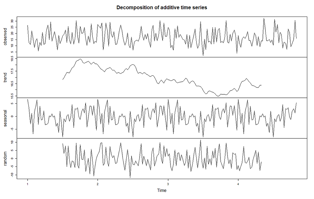
Interestingly, there seems to be a general downward trend on sales. Looking at the smaller range of the vertical axis for seasonality, we can see that weekly seasonality effects are rather tiny compared to the other components like trend.
Let’s now fit our marketing mix model, this time using tslm() instead of lm() and including trend and seasonality to see if we can improve the model.
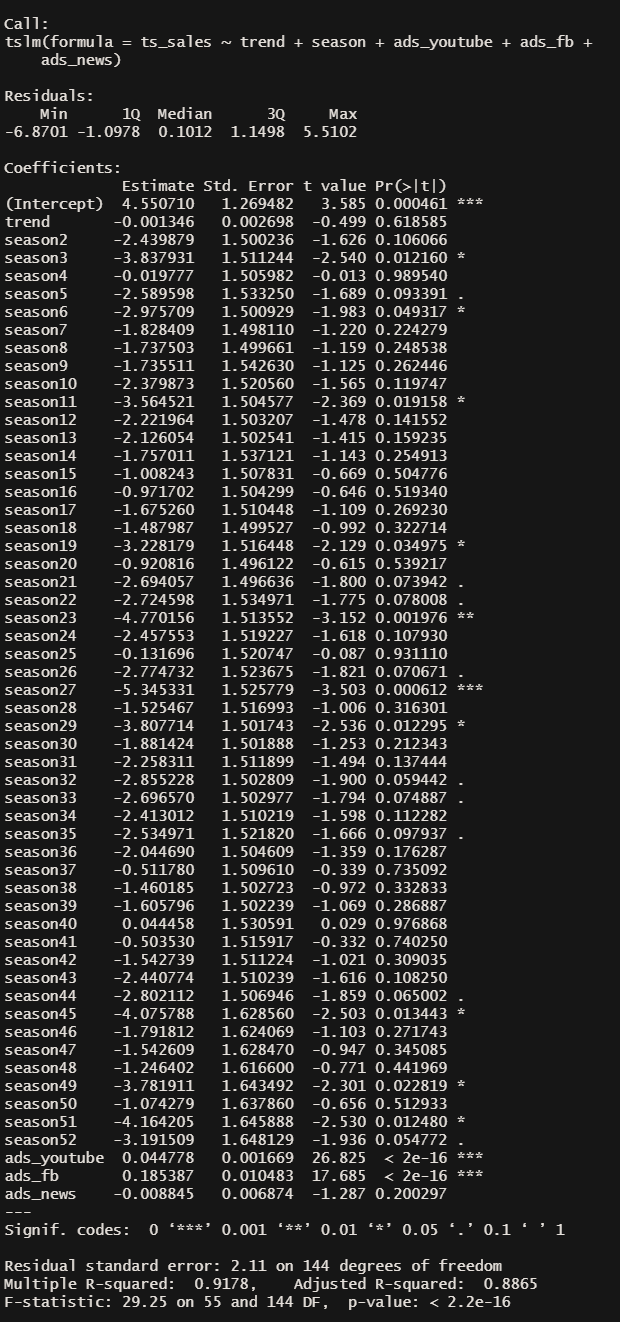
Yes the model has improved slightly!
Very small changes in coefficient estimates for Youtube and Facebook, t-statistic are still high (above 2) with statistically significant p-values for both which means we can remain confident with our inferences here (💡 again, reminding ourselves that the figures are in the 1000s !!) i.e for every £1000 spent on Youtube, we can expect sales to increase by about 45 (0.045*1000) units. For every £1000 spent on Facebook, we can expect sales to increase by 185 (0.185 * 1000) units.
Notice that tslm() have used dummy variables for seasonality and week 1 is not included — this is because week 1 is being used as the comparison against our seasonal coefficient estimates, allowing us to interpret in this way: sales in week 2 have decreased by 2,430 (2.43*1000) units compared to week 1. Sales in week 3 have decreased by 3,840 (3.84*1000) units compared to week 1. And so on.
Most of the coefficient estimates for seasonality have not got large enough t-statistics (above 2) and p-values are not significant. Only weeks 23 and 27 appear to have t-statistics above 2 with highly significant p-values, both are saying that sales have decreased compared against week 1.
R² goodness-of-fit of the model have also improve slightly from 0.88 in the previous model to 0.89 in the current one.
Other Considerations
Broadly however, the outcome here does not look good. Sales are generally following a downward trend. We know Youtube and Facebook appear to drive good return, newspaper not so. Perhaps we can experiment with pulling back on newspaper ads next time?
Predict
Let’s imagine we have presented these early findings. The client appreciates the model is not 100% perfect and this is a project that is continuously being improved upon.
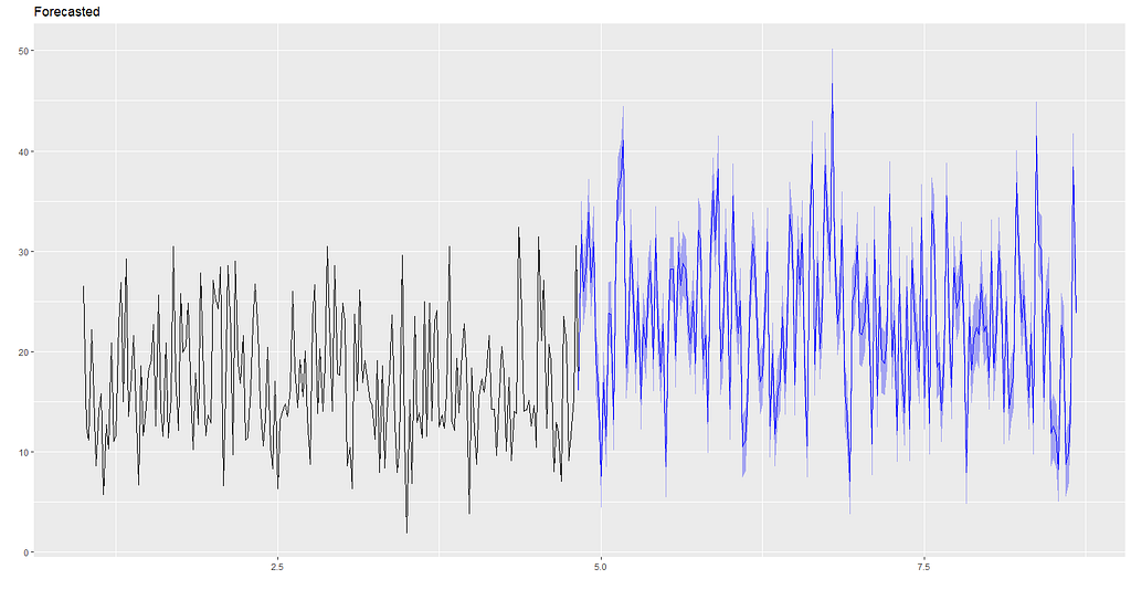
If there were no changes to ad budgets and channels, and we assume trend and seasonality remain similar for the next period, using our model we’d expect performance to look like this:
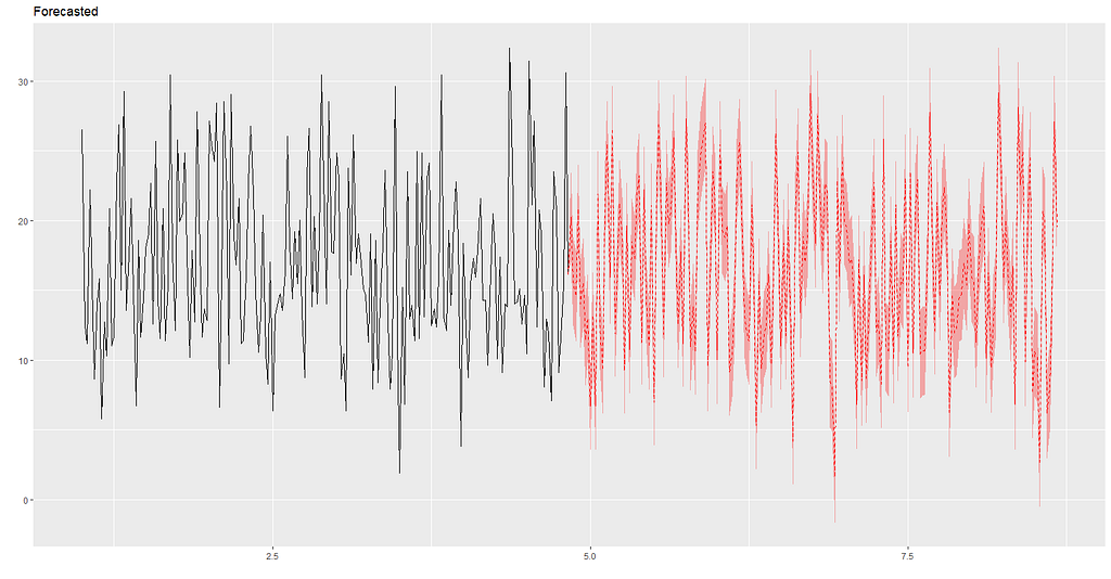
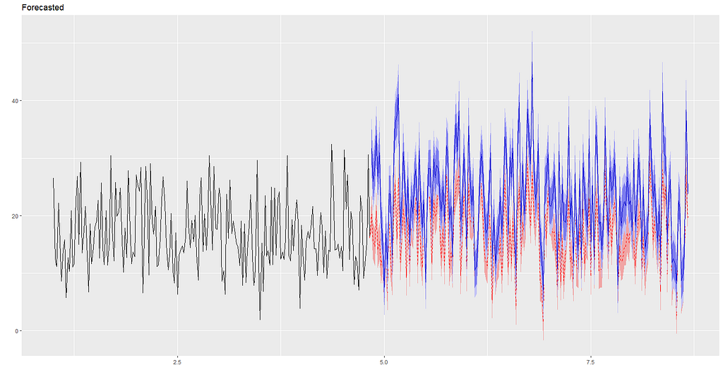
However if the client is open to our suggestion to pull back on Newspaper ads, and re-assign it as additional budget for Youtube and Facebook: 40% to Youtube and 60% to Facebook (this is applied on top of their current budgets which we will assume will be the same as they have been), using the model, sales performance is forecasted to look like this:
Overlaying the two graphs together it would appear the budget re-allocation from newspaper to Youtube and Facebook could potentially improve sales performance🤑🤑!
Another thing to point out is that with digital channels, we can track current run-rates against forecast almost in realtime or at the very least, daily, which means experimenting, ad-testing, changing direction (if we need to), performance monitoring and optimisation can be done seamlessly.
To get fitted values from the model, simply call:
forecast_new_spends$fitted
Going Further
There are clearly other factors here that have not been included that could also impact the effectiveness of the model. For example, we have only reviewed 3 channels, were there other marketing activities we have missed? We did not include other variables like weather or if discounts were on, perhaps we should also include whether there were holidays in specific weeks. Consider exploring other frequency options such as quarterly, or monthly.
We may also wish to consider other models and compare it against the simple multiple regression method we have used here.
Due to the already long length of this article and lack of time, I have not been able to cover the process for training and testing the model this time round. Perhaps we can cover this and comparisons with other models in a future post, time permitting!! 🐱🏍
The End
Thanks for reading this far and if there is anything I have missed, or if there are better ways of approaching the issues I have discussed earlier do share in the comments. It’s great to learn together :)
Full R Code
👉 Get the full R code from my Github repo here.
References
Broadbent, S., 1979. One Way TV Advertisements Work, Journal of the Market Research Society, 23(3).
Marketing data sample used in this post is from the Datarium package for R licensed under GPL-2 General Public License https://www.rdocumentation.org/packages/datarium/versions/0.1.0
R is a free open source statistical software https://www.r-project.org/
Using R to Build a Simple Marketing Mix Model (MMM) and Make Predictions was originally published in Towards Data Science on Medium, where people are continuing the conversation by highlighting and responding to this story.
from Towards Data Science - Medium https://ift.tt/3nJsa43
via RiYo Analytics


No comments