https://ift.tt/3mR4aeI Practical applications of the Fourier transform Now we have all the tools we need to need to demonstrate some real-...
Practical applications of the Fourier transform
Now we have all the tools we need to need to demonstrate some real-world use cases for FFTs!
Check out the previous articles in the series!
- https://towardsdatascience.com/the-fourier-transform-1-ca31adbfb9ef
- https://towardsdatascience.com/the-fourier-transform-2-understanding-phase-angle-a85ad40a194e
- https://towardsdatascience.com/the-fourier-transform-3-magnitude-and-phase-encoding-in-complex-data-8184e2ef75f0
Introducing the IFFT
So far, we’ve treated the Fourier transform as a mathematical black box operation. Similarly, we’ll now introduce the inverse Fourier transform without dissecting the implementation details. The inverse Fourier transform (IFFT) lets us reverse the FFT!
The inverse Fourier transform is the mathematical operation that maps our function in the frequency domain to a function signal in the temporal or spatial domain.
Critically, this inverse operation allows us to jump between the frequency domain and the temporal/spatial domain, manipulating our data in whichever is most convenient.
Applications of the Fourier transform
Let’s start toying with real-world applications of the Fourier transform!
Filtering and denoising
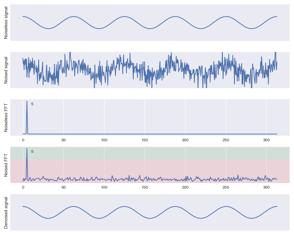
FFTs provide us with invaluable “denoising” techniques to suppress or remove artifacts from data. To start, let’s consider an approximately stationary signal that is subject to some low-power white noise. For demonstration, we can use the same pure tone signal we used before (Figure 1, “noiseless signal”). In addition, though, let’s add some Gaussian noise to that signal (Figure 1, “noised signal”).
Just as we did previously, we can use the Fourier transform to look at the frequency components (Figure 1, “Noiseless FFT” and “Noised FFT”).

Super interesting! In the FFT, we can see some properties of the noise I chose to add. The Gaussian noise I added was zero mean additive “white” noise: it had roughly equal intensity across frequencies.
Even though the noise looks pretty grisly in the temporal domain, it is easy to separate out in the frequency domain. Looking at the magnitude values of our Fourier transform allows us to visualize the amplitude as a function of frequency. In this simple case, we can perfectly recover our noiseless signal pretty easily! Since we have clean separation between the signal and the noise, we can set a hard threshold and drop (i.e. set to zero) low amplitude components. Keeping the values above the threshold (Figure 1, “noised FFT” in green) and dropping the values before the threshold (Figure 1, “noised FFT” in red), we get a great reconstruction of the signal without noise (Figure 1, “Denoised signal”)!
We usually don’t end up getting quite so lucky. Real-world noise can be lot nastier! In many cases, the noise might be louder than our signal. There are lots of other approaches we can use, though!
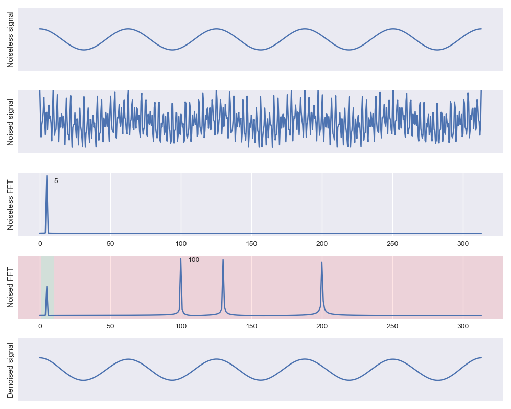
To touch on one common filtering method, let’s take a look at the bandpass filter. A bandpass filter is composed of two thresholds: (1) a filter that removes frequencies below some threshold, allowing higher frequencies to pass (i.e., “high pass”) and (2) a filter that removes frequencies above some threshold, allowing lower frequencies to pass (i.e., “low pass”). In combination, these two filters only allow a “band” of frequencies between a low frequency cutoff and a high frequency cut off to pass.
Let’s add some high frequency components to our signal. In practice, these might be unwanted artifacts of our environment (e.g., uncontrolled audio source in the environment for our sound example).

Now, rather than setting a hard threshold on the minimum amplitude, we’ll set components to zero for frequencies outside of our passband (Figure 2, “noised FFT”). Once again, we recover our signal from the noise!
Feature extraction
We can also use the Fourier transform to pull out characteristics of our data. If you’ve encountered the idea of wavelet convolution before, there is a deep mathematical connection! Let me know if you are interested in the comments of an article exploring the convolution theorem in depth!
For now, though, we can focus on a simple example by visualizing different frequency components. While we’re at it, let’s try our hand at a 2D generalization of the Fourier transform!
All the intuitions we’ve built still apply! Values near the origin will correspond to low frequencies and values far from the origin will correspond to high frequencies. As before, np.abs will recover magnitudes and np.angle will recover phase.
If we want to inspect just the edges in an image, we can take a look at the high frequency values, setting the amplitude of Fourier transform components near the origin to zero (Figure 4).

We can also look at just the slow-changing low frequency components by setting the values farther from the origin to zero!

We can use these sorts of tricks to extract all sorts of interesting statistical properties. The same methods apply to one-dimensional temporal or spatial data, as well, allowing us to separate slow-moving low-frequency trends from sudden abrupt changes in timeseries data (e.g., stock values or overall market analytics).
Other applications
There are countless other uses, but here are a few that come to mind if you are interested in further reading:
- Lossy image compression (like JPEG) often uses a transform to the frequency domain under the hood,
- Physical system modeling (like thermodynamics! Aside, 3blue1brown is an absolute inspiration),
- Alignment and registration methods to get photos (or timeseries data!) lined up,
- Estimation and prediction of periodic biological phenomena (e.g., breathing rate, heart rate), and
- Radio data analysis and processing.
We’ve learned enough about the Fourier transform to be dangerous! We’ve managed to develop our intuitions sufficiently and can solve real-world problems. If there are other Fourier concepts you’d like to see explained, leave a comment. Thanks for reading!
Up next, we’ll introduce a Fourier “cheat sheet” of common operations and their place in your toolkit.
The Fourier Transform (4): Putting the FFT to work was originally published in Towards Data Science on Medium, where people are continuing the conversation by highlighting and responding to this story.
from Towards Data Science - Medium https://ift.tt/3FU0nov
via RiYo Analytics

ليست هناك تعليقات