https://ift.tt/3zNIc1L Getting Started with Causal Inference Going beyond “Correlation is not Causation” and understanding the “why” Pho...
Getting Started with Causal Inference
Going beyond “Correlation is not Causation” and understanding the “why”

Throughout the journey of technological innovation, the most coveted goal of companies is to find ways to change human behavior, by answering questions such as, “How can I make visitors become customers?”, “Does this discount coupon help?”, “Which campaign results in better engagement and profits?”, etc. This needs working with the data to develop reliable actionable prescriptions, more specifically to understand what should be done to move our key metrics in the desired direction.
Data scientists have been using predictive modelling to generate actionable insights, and these models are great at doing what they are meant to do, that is, to generate predictions, but not so on providing us with reliable actionable insights. A lot of them suffer from spurious correlations and different kinds of biases, which we are going to discuss in this article.
So, why do we need causal inference? The answer lies in the question itself because we need to know the “WHY”, why is something happening?, for example, “Are sales increasing because of coupon code?”. Causal inference is the Godfather of actionable prescriptions. It’s not something new, economists have been using it for years to answer questions like, “Does immigration cause unemployment? “, “What is the impact of higher education on income?” etc.
ASSOCIATION VS CAUSATION?
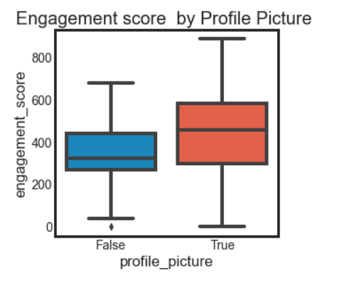
We have often heard statements like “Association is not causation”, and it’s intuitively understandable also. Now let’s develop some mathematical perspective on this. Suppose, someone tells you that people who have a profile picture on a social media site have better engagement, so to increase engagement, we should ask users to upload a profile picture. One can quickly point out it’s probably the case that users with more friends have a profile picture, and prompting users with the “People you may know option” is a better way of increasing engagement. Profile picture is not causing engagement in this case, it is just associated with engagement.
Before we get started with the mathematics, let’s understand a few terms which we will be using throughout this article, Treatment, and Control. Treatment is nothing but some sort of intervention for which we want to know the effect. In our case, having a profile picture is treatment.
Treatment ={1, if unit i is treated and 0 otherwise}
Yᵢ is the outcome for unit i , Y₁ᵢ is the outcome with treatment for unit i, and Y₀ᵢ is the outcome without treatment. The fundamental problem with Causal inference is that we don't observe Yi for both treatment and control. Therefore the individual treatment effect is never observed, there are ways to estimate that, but since we are just getting started, let’s focus on the Average Treatment Effect (ATE)
ATE = E[Y₁-Y₀]
ATT = E[Y₁-Y₀|T=1], Average treatment effect on the treated.
Intuitively we understand what makes association different from causation for certain cases, but there is a one-word answer for this, and it’s called Bias. In our example, people without profile pictures might have fewer friends and/or are from a higher age group. Since we can only observe one of the potential outcomes, it is to say, Y₀ of treated is different from Y₀ of untreated. Y₀ of treated is higher than Y₀ on untreated, that is people with a profile picture(treatment) will have higher engagement without it as they might be younger and more tech-savvy and have more friends. Y₀ of treated is also called counterfactual. It’s something we don't observe, but only reason about. Now with this understanding, let’s take another example, "Does private school education lead to higher wages as compared to public school?". We have the understanding to say that students going to Private school have richer parents, who are probably more educated because education is related to financial wealth, rather than just implying causation because there seems to be an association between higher wages and private school education.
Association is given by = E[Y|T=1]-E[Y|T=0]
Causality by = E[Y₁-Y₀]
Replacing with observed outcome in association equation
E[Y|T=1]-E[Y|T=0] = E[Y₁|T=1]-E[Y₀|T=0]
Adding and subtracting the counterfactual outcome E[Y₀|T=1](outcome of treated units, had they not been treated)
E[Y|T=1]-E[Y|T=0] = E[Y₁|T=1]-E[Y₀|T=0]+E[Y₀|T=1]-E[Y₀|T=1]
E[Y|T=1]-E[Y|T=0] = E[Y₁-Y₀|T=1] + {E[Y₀|T=1]-E[Y₀|T=0]}Bias
Association = ATT +Bias
This is God’s equation of the Causal universe. It tells us why association is not causation and the bias is given by how much the treatment and control group differ before the treatment when neither of them has received the treatment. If E[Y₀|T=1]=E[Y₀|T=0], that is there is no difference between treatment and control before the treatment is received, then we can infer Association is Causation.
Causal inference techniques are aimed at making treated and control groups similar in all ways except the treatment. Randomized Control Trials(RCT) or randomized experiments are one such way of making sure the Bias term is zero. It involves randomly assigning units to treatment or control group, such that E[Y₀|T=1]=E[Y₀|T=0].A/B testing is a randomized experiment, a technique widely used by companies like Google and Microsoft, to find the impact of changes to the site in terms of user experience or algorithms. But it’s not always possible, in our example, we can not randomly give the option to upload profile pictures to users, or we can’t ask people to smoke to quantify the impact of smoking on pregnancy, etc. Also, it is not something that can be used with non-random observational data.
Before we get into some of the ways to make sure the treatment and control group are similar in all ways except for the treatment, let’s first look into Causal graphs, the language of Causality.
Causal Graphs: Language of Causality
The basic idea of a causal graph is to represent the data generating process. Sounds simple? Not really, though! It requires us to know beforehand all the possible factors which can affect the outcome, treatment being one of them.
A very common example is the impact of medicine on the survival rate of patients. If the medicine is given to people who are severely affected by the disease, that is, if the treatment consists of severely ill patients and the control group has less severely ill patients, it would introduce a bias in our design.
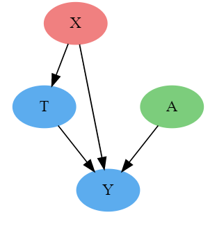
One way of reducing this bias is to control for other factors like the severity of the disease(randomly allocate treatment to different levels of severity). By conditioning on severe cases, the treatment mechanism becomes random. Let’s represent this in the causal diagram.
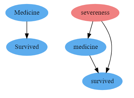
A causal diagram consists of nodes and edges. The nodes represent different factors and outcomes, and edges represent the direction of causality. In Fig A above, the medicine causes patients’ survival, and in Fig B, severity and medicine both cause patients’ survival, while severity also causes treatment. These diagrams are useful because they tell if two variables are related to each other and the paths(arrow between the nodes) give us the direction of the relationship
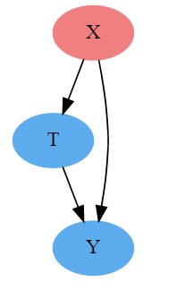
This brings us to the idea of Good paths and Bad paths. Good paths Or Front doors are the reason why the treatment is related to outcome, and this is what our analysis is interested in. Usually, these are the paths where the arrow faces away from treatment, rest all the paths are bad paths or back doors, for which we need to control, usually the path where arrows point towards the treatment. Pretty evident in the example above. Isn't it?
Closing back doors, or controlling or conditioning on variables that affect the treatment are just some of the other words for making sure bias is zero and our causal inference results are more valid. We call this bias Confounding, which is the big baddie of the Causal Universe. Confounding occurs when there is a common factor affecting treatment and outcome, so to identify the causal effect, we need to close the backdoor, by controlling for the common cause. In our example above, severity is introducing confounding, so unless we control for severity we cannot get a causal estimate of medicine on patients’ survival(T -> Y).
Should we control for everything to make sure our model doesn't suffer from confounding bias? Wish life in the causal universe was that simple!
Imagine we want to get the impact of practice in chess on working memory. We have somehow randomized the measure of practice such that E[Y0|T=1]-E[Y0|T=0] = 0. Since the measure of practice is randomized, we can directly measure the causal impact without controlling for any variable. However, if we decide to control on performance in actual games, we are adding selection bias to our estimate. By conditioning performance, we are looking at groups of players with similar performance, while not allowing working memory to change much, as a result, we don't get a reliable impact of practice on working memory. We have a case where E[Y₀|T=0, Per = 1]>E[Y₀|T=1, Per =1 ], i.e., people who have better performances without much much practice probably have better working memory.
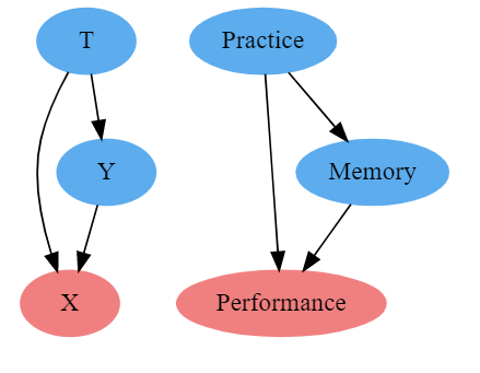
Confounding bias occurs when we fail to control for the common cause of treatment and outcome. Selection bias occurs when we control for the common effect of treatment and outcome (as in the example above) or when we control for variables in the path from cause to effect(Discussed with example in regression case 3 below)
We have talked a lot about it in theory, but how do we implement this? How do we control for variables after the data has already been collected to get the impact of Treatment?
REGRESSION TO THE RESCUE
Regression is like the Caption America of Data Science universe, solving problems and creating value from data long before the ensembles and neural networks became mainstream. Regression is the most common way of identifying causal effects, quantifying the relationship between variables, and closing the back doors by controlling for others.
If you are not familiar with regression, I suggest you go through that first. There are hundreds (if not thousands) of books and blogs written on regression, just one google search away. Our focus will be more on using regression for identifying causal impact.
Let’s see how this works in practice. We have to get the impact on email campaign on sales, more specifically we want to estimate the model
Sales = B₀+B₁*Email + error.
The data is random, that is there is no bias, E[Y₀|T=1]-E[Y₀|T=0]=0.
We can directly calculate out ATE
(df.groupby("Email")["Sales"].mean())
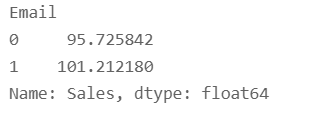
Since this is random data, we can directly calculate ATE = 101.21–95.72=5.487. Now let’s try regression on this.
result = smf.ols('Sales ~ Email', data=df).fit()result.summary().tables[1]
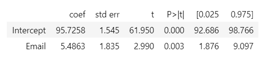
This is pretty cool, right? We not only get ATE as the coefficient of Email but also get confidence intervals and P values. The intercept gives us values of Sales when Email=0, i.e., E[Y|T=0], and the Email coefficient gives us ATE E[Y|T=1]-E[Y|T=0].
It is easier to get a causal estimate for random data, as we don't have to control for bias. As we have discussed above, it is a good idea to control for confounders, but we should be careful of selection bias as we keep increasing the number of variables that we control. In the next few sections, we will discuss about which variables should we control for in our causal estimation efforts and implement them using Regression.
Case 1: Controlling for confounders.
In the absence of random data, we cannot get unbiased causal impact without controlling for confounders. Suppose we want to quantify the impact of an additional year of education on hourly wage. This is our data
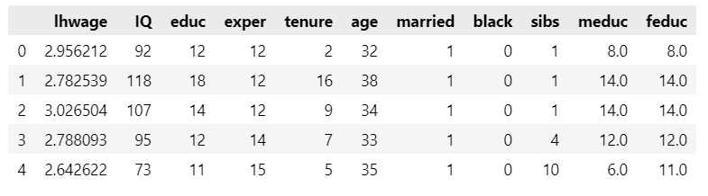
Let’s see the results with this simple model
log(lhwage) = B₀+ B₁*educ + error
result = smf.ols('lhwage ~ educ', data=wage).fit()
result.summary().tables[1]
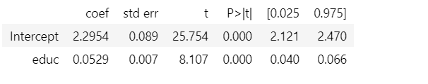
Since this is a log model, for every 1-year increase in education, the hourly wage is expected to increase by 5.3%. But does this model suffer from any bias? Is E[Y₀|T=1]-E[Y₀|T=0] =0 ? Since this is non-random data from an experiment, we can argue that people with more years of education have richer parents, a better network, or maybe they belong to a privileged social class. We can also argue that age and years of experience also affect wages and years of education. These confounding variables which affect our treatment and education introduce a bias (E[Y₀|T=1]-E[Y₀|T=0] !=0) in our model design for which we need to control. Let’s add these controls to our model and see the results.
controls = ['IQ', 'exper', 'tenure', 'age', 'married', 'black', 'sibs', 'meduc']
result = smf.ols('lhwage ~ educ +' + '+'.join(controls), data=wage).fit()
result.summary().tables[1]
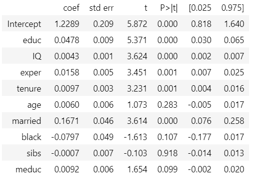
As you see above, the impact of education on hourly wage has decreased to 4.78% after accounting for controls. This confirms that the first model without any control was biased, overestimating the impact of years of education. This model is not perfect, there might be still some confounding variables that we have not controlled for, but it’s definitely better than the previous one.
Causal inference with observational data (non-random) requires internal validity, we have to make sure we have controlled for variables that can contribute to bias. This is different from the external validity required for a predictive model which we implement using a train test split to get reliable predictions(not causal estimates).
Case 2: Controlling for predictors to reduce standard errors
We have seen above how adding controls for confounders can give us more reliable causal estimates. But what other variables should we add to the model? Should we add variables that are good at capturing the variance in the outcome, but are not confounders? Let’s answer that with an example
Suppose we ran an email campaign to promote our grocery store. The emails were randomly sent, and there is no bias, i.e., no other variable affects our treatment allocation, and E[Y₀|T=1]-E[Y₀|T=0] =0. Let’s work out the effect of email on sales.
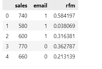
model = smf.ols('sales ~ email', data=email).fit()
model.summary().tables[1]
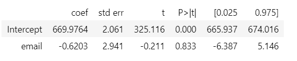
It looks like the email campaign has a negative effect on sales. The coefficient has high standard errors and it isn't significant. Let’s dig deeper and see the variability in sales for treatment (email) and control(no email)
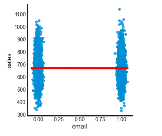
Since this data comes from a random experiment, assignment of email is done through a flip coin, no other variable is affecting the treatment. But we see there is a huge variance in sales. It is probably that email has a very little effect on sales and people who are recent, frequent, and heavy buyers (RFM values) are dictating the sales. That is we can say the variability of sales is affected by other factors like rfm score of users or seasonality if the products are seasonal like winter clothes. So need to control for these effects, to get a reliable estimate of the causal impact of our email campaign. Let bring in the rfm score in our model.
model = smf.ols('sales ~ email + rfm', data=email).fit()
model.summary().tables[1]
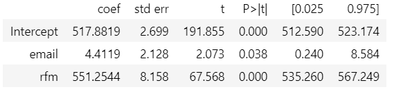
Adding rfm has resulted in a positive impact of email on sales and the email variable is also significant at 95% level. So controlling for variables that have high predictive power helps in capturing the variance, and provides more reliable causal estimates. Basically, in the above example, when we look at similar customers(similar levels of rfm score), the variance in the outcome variable is smaller.
To summarize Case1 and Case2, we should always control for confounders and variables that have great predictive powers in our causal design.
Case 3 : Bad controls leading to Selection Bias
In the era of the data boom, there is no shortage of variables that we can just push into our model. We discussed above that we shouldn't be adding all the variables to the model, or else we introduce another kind of bias known as selection bias.
Suppose, we want to know the impact of a college degree on wages. We have somehow managed to randomize college degrees (1 for college education and zero otherwise). If we now control for white-collar jobs in our design we are introducing selection bias. We close the front door path along which the college education impacts wages.
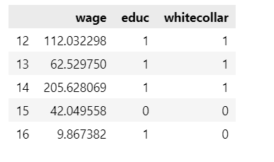
model = smf.ols('wage ~ educ', data=df).fit()
model.summary().tables[1]
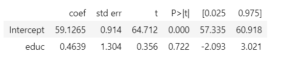
College education has a positive impact on wages, people with college education on average earn 0.46 units higher than without it.
model = smf.ols('wage ~ educ + whitecollar', data=df).fit()
model.summary().tables[1]
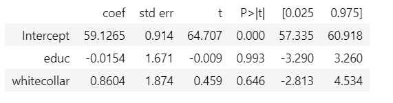
Controlling for white-collar jobs has resulted in selection bias by closing one of the channels through which a college degree affects wages. This results in underestimation of the impact of a college degree on education. We expect E[Y₀|T=1]-E[Y₀|T=0] =0 because of randomization, however after controlling for white-collar job E[Y₀|T=0, WC=1] > E[Y₀|T=1, WC=1], that is, people who have white-collar jobs even without a college degree are probably more hard-working than those who need a college degree for it.
Regression is very effective and somewhat magical in controlling for confounders. The way it does it is by partitioning the data into confounder cells, calculating the effect in each of the cells, and combining them using a weighted average where weights are the variance of treatment in the cell.
But everyone has their own issues, and so does regression. It doesn't work with nonlinearity, and since it uses the variance of treatment in groups as weights, ATE is more affected by high variance factors. But this is not the only tool we have under our belt, there are other methods all aimed at making treatment and control groups similar, which we will discuss in part 2 of this series.
References
- https://matheusfacure.github.io/python-causality-handbook/
- https://www.bradyneal.com/causal-inference-course
- https://theeffectbook.net/
- https://www.masteringmetrics.com/
- https://www.amazon.in/Applied-Data-Science-Transforming-Actionable/dp/0135258529
Getting started with Causal Inference was originally published in Towards Data Science on Medium, where people are continuing the conversation by highlighting and responding to this story.
from Towards Data Science - Medium https://ift.tt/3HV8KAT
via RiYo Analytics


No comments