https://ift.tt/31lv0DQ Using PyCaret Time Series Module Photo by Isaac Smith on Unsplash 📚 Background When building a model for any...
Using PyCaret Time Series Module

📚 Background
When building a model for any machine learning problem, we must pay attention to bias-variance tradeoffs. Specifically, for time series:
- Having too much bias (underfitting) means that the model is not able to capture all the signals in the data and hence leads to a higher error during the training phase (and in turn during the prediction phase as well).
- Having too much variance (overfitting) in the model means that the model is not able to generalize well to unseen future data (i.e. it can do well on the training data but is not able to predict the future data as well as it trained).
Let’s see how this can be diagnosed with PyCaret.
🚀 Solution Overview in PyCaret
The solution in PyCaret is based on the recommendation by Andrew Ng [1]. I would highly recommend the readers go through this short video first before continuing with this article. The steps followed in PyCaret are:
- The time-series data is first split into train and test splits.
- The train split is then cross-validated across multiple folds. The cross-validation error is used to select from multiple models during the hyperparameter tuning phase.
- The model with the best hyperparameters is trained on the entire “training split”
- This model is then used to make predictions corresponding to the time points in the “test split”. The final generalization error can then be reported by comparing these “test” predictions to the actual data in the test split.
- Once satisfied, the user can train the entire dataset (train + test split) using the “best hyperparameters” obtained in the previous steps and make future predictions.
1️⃣ Setup
We will use the classical “airline” dataset [6] to demonstrate this in PyCaret. A Jupyter notebook for this article can be found here and also at the end of the article under the “Resources” section.
from pycaret.datasets import get_data
from pycaret.internal.pycaret_experiment import TimeSeriesExperiment
#### Get data ----
y = get_data(“airline”, verbose=False)
#### Setup Experiment ----
exp = TimeSeriesExperiment()
#### Forecast Horizon = 12 months & 3 fold cross validation ----
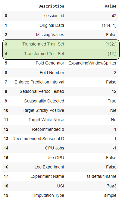
exp.setup(data=y, fh=12, fold=3, session_id=42)
2️⃣ Train-Test Split
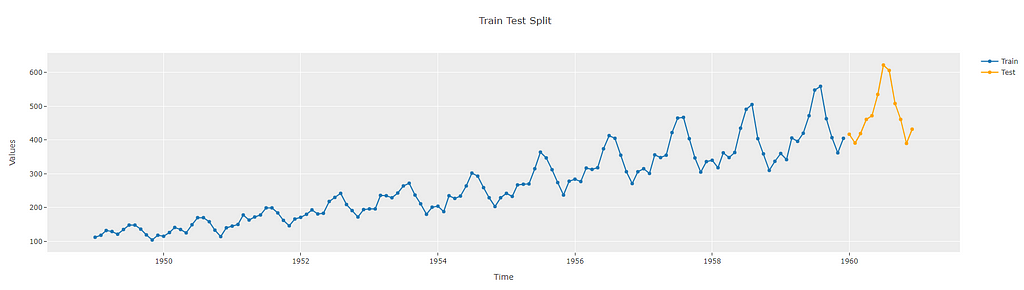
To diagnose bias-variance tradeoffs, PyCaret initially splits the time series data into a train and test split. The temporal dependence of the data is maintained when performing this split. The length of the test set is the same as the forecast horizon that is specified while setting up the experiment (12 in this example). This is shown in the setup summary.
This split can also be visualized using the plot_model functionality.
exp.plot_model(plot="train_test_split")
3️⃣ Cross-Validation
Next, the training split is broken into cross-validation folds. This is done so that the training is not biased by just one set of training data. For example, if the last 12 months in the data were an anomaly (say due to Covid), then that might impact the performance of an otherwise good model. Alternately, it might make an otherwise bad model look good. We want to avoid such situations. Hence, we train multiple times over different datasets and average the performance.
It is important to again maintain the temporal dependence when training across these multiple datasets (also called “folds”). Many strategies can be applied like expanding or sliding window strategies. More information about this can be found in [2].
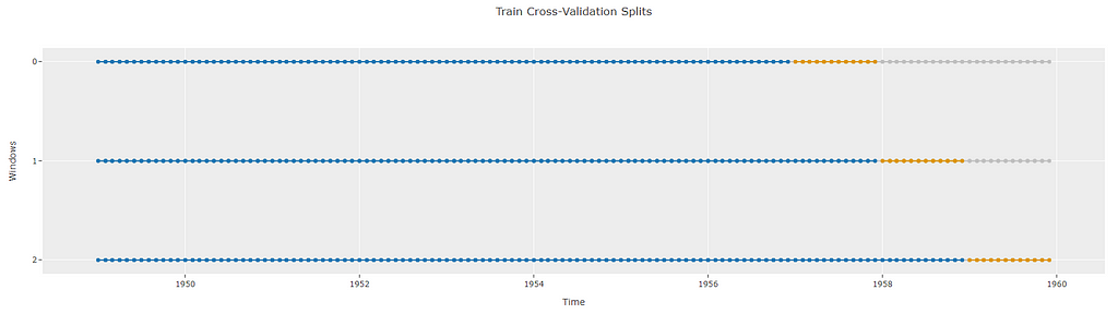
The number of folds can be controlled during the setup stage. By default PyCaret time series module uses 3 folds. The folds in the training data can be visualized using plot_model again. The blue dots represent the time points that are used for training in each fold and the orange dots represent the time points used to validate the performance of the training fold. Again, the length of the orange dots is the same as the forecast horizon (12)
exp.plot_model(plot="cv")
4️⃣ Creating Initial Model
We will take the example of a reduced regression model for this article. More information about reduced regression models can be found in [3].
model = exp.create_model("lr_cds_dt")
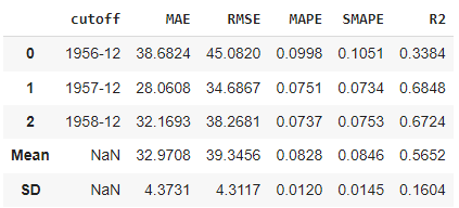
The performance is displayed across the 3 folds. The average Mean Absolute Error (MAE) across the 3 folds is > 30 and the Mean Absolute Percentage Error (MAPE) is > 8%. Depending on the application, this may not be good enough.
Once the cross-validation is done, PyCaret returns the model that is trained on the entire training split. This is done so that the generalization of the model can then be tested on the test dataset that we held out previously.
exp.predict_model(model)
exp.plot_model(model)
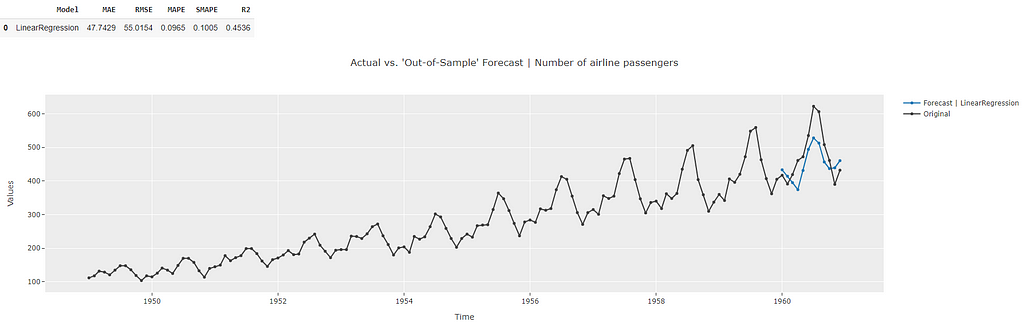
Prediction using this model now shows the forecasts for the time points corresponding to the test dataset (blue line). The metrics for these “test” forecasts are also displayed. These are worse than the metrics obtained during the cross-validation. Since the metrics were bad to begin with (high cross-validation errors), this is indicative of a high bias in the model (i.e. the model is not able to capture the trends in the dataset well at this point). Also, the test metrics are worse than the cross-validation metrics. This is indicative of high variance (refer to [1] for details). This is also visible in the prediction plot as well which shows that the blue prediction line is not close to the corresponding black line during the test period.
Let’s see if we can improve the bias by tuning the model’s hyperparameters.
5️⃣ Tuning the Model to Improve Performance
The tuning process tries various hyperparameter combinations to see which ones fit the model the best. More information can be found in [4] and [5]. Once the various hyperparameter combinations are tried out, the best hyperparameters are picked based on the mean cross-validation error across the “folds”. The cross-validation metrics using these best hyperparameters are then displayed.
tuned_model = exp.tune_model(model)
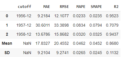
So, we have been able to reduce the errors during the cross-validation stage to approximately <= 20 and the MAPE is < 5% by performing hyper-parameter tuning. This is much better than before and we have reduced the underfitting significantly. But now we need to ensure we are not overfitting the data. Let’s look at the performance across the test dataset again.
exp.predict_model(tuned_model)
exp.plot_model(tuned_model)
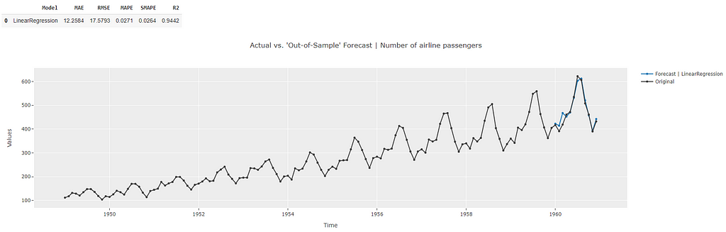
The forecasts across the test dataset show better performance than the cross-validation metrics indicative of a lack of overfitting. The plot also shows a good match to the actual data points during the test period.
So this model looks good. But what we need is the ability to predict the true “unknown” future data. This can be done by finalizing the model.
6️⃣ Finalizing the Model to make Future Predictions
Finalizing the model takes the hyperparameters from the model (tuned_model in this case), and fits the entire dataset using these hyperparameters.
final_model = exp.finalize_model(tuned_model)
print(exp.predict_model(final_model))
exp.plot_model(final_model)

And there you have it. Our best model is now able to make future predictions. Note that metrics are not displayed at this point since we do not know the actual values for the future yet.
🚀 Conclusion
Hopefully, this workflow example has shown why it is important to diagnose bias-variance tradeoff. For time series, this process is complicated by the fact that the temporal dependence must be maintained when performing the splits and cross-validation. Luckily, the PyCaret Time Series module makes managing this process a breeze.
That’s it for this article. If you would like to connect with me on my social channels (I post about Time Series Analysis frequently), you can find me below. Happy forecasting!
📘 GitHub
📗 Resources
- Jupyter Notebook containing the code for this article
📚 References
[1] Model Selection and Training/Validation/Test Sets by Andrew Ng.
[2] Time Series Cross Validation in PyCaret
[3] Reduced Regression Models for Time Series Forecasting
[4] Basic Hyperparameter Tuning for Time Series Models in PyCaret
[5] Advanced Hyperparameter Tuning for Time Series Models in PyCaret
[6] Airline Dataset available through sktime python package under BSD 3-Clause License.
Bias-Variance Tradeoff in Time Series was originally published in Towards Data Science on Medium, where people are continuing the conversation by highlighting and responding to this story.
from Towards Data Science - Medium https://ift.tt/3IerCf2
via RiYo Analytics

No comments