https://ift.tt/3wIY2c8 Defending against adversarial examples with GloRo Nets Photo by Henrique Ferreira on Unsplash Over the last se...
Defending against adversarial examples with GloRo Nets

Over the last several years, deep networks have extensively been shown to be vulnerable to attackers that can cause the network to make perplexing mistakes, simply by feeding maliciously-perturbed inputs to the network. Clearly, this raises concrete safety concerns for neural networks deployed in the wild, especially in safety-critical settings, e.g., in autonomous vehicles. In turn, this has motivated a volume of work on practical defenses, ranging from attack detection strategies to modified training routines that aim to produce networks that are difficult — or impossible — to attack. In this article, we’ll take a look at an elegant and effective defense I designed with my colleagues at CMU (appearing in ICML 2021) that modifies the architecture of a neural network to naturally provide provable guarantees of robustness against certain classes of attacks — at no additional cost during test time.
We call the family of neural networks protected by our approach “GloRo Nets” (for “globally-robust networks”). For those interested in experimenting with the ideas presented in this article, a library for constructing and training GloRo Nets is publicly available here.
Motivation: Adversarial Examples
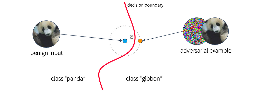
While deep neural networks have quickly become the face of machine learning due to their impressive ability to make sense of large volumes of high-dimensional data and to generalize to unseen data points, in as early as 2014, researchers were beginning to notice that deep networks can easily be fooled by making imperceptible modifications to their inputs. These perturbed inputs that successfully cause erroneous behavior have been termed adversarial examples. A classic illustration of an adversarial example is shown below.

Broadly speaking, for an input to be considered an adversarial example, it should resemble one class (e.g., “panda”), while being classified as another class (e.g., “gibbon”) by the network. This suggests that the perturbations to the input should be semantically meaningless. This requirement is rather nebulous, and inherently tied to human perception; it may mean that changes are imperceptible to the human eye, or simply that they are inconspicuous in the given context. Thus, we often consider more well-defined specifications of adversarial examples; most frequently, small-norm adversarial examples.
An adversarial example is small-norm if its distance (according to some metric, e.g., Euclidean distance) from the original input is below some small threshold, typically denoted by ε. Geometrically, this means that the original point is near a decision boundary in the model, as shown in the figure below. In terms of perception, when ε is sufficiently small, any points that are ε-close to the original input will be perceptually indistinguishable from the original input, meaning that small-norm adversarial examples fit our broader requirements for adversarial examples.
While the precise reasons behind the existence of adversarial examples is not the focus of this article, some high-level intuition might give a bit of an idea of why this phenomenon is so pervasive in deep networks. Essentially, we can consider the decision surface of the network, which maps the network’s output as a function of its input. If the decision surface is steep in some direction, the network will quickly change its mind on the label it assigns to an input as the input is modified slightly in that direction. As deep networks typically operate in very high-dimensional space (often thousands of dimensions), there are many different directions in which the decision surface is potentially steep, making the chance that any point is near an unexpected “cliff” more likely than not.
Defending Against Adversaries
Numerous defenses have been proposed to deal with the threat of adversarial examples — particularly small-norm adversarial examples. While many of these approaches are heuristic in nature — that is, they do not provide guarantees that tell us when, or if, the model’s predictions cannot be manipulated — in the most safety-critical applications, this may not be good enough. For our purposes, we are interested in provable defenses.
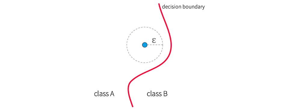
The first question is, what, precisely, do we want to prove? In the case of small-norm adversarial examples, the property we are after is what is called local robustness. Local robustness on a point, x, stipulates that all points within a distance of ε from x are given the same label as x. Geometrically, this means that a ball of radius ε around x is guaranteed to be clear of any decision boundaries, as shown in the figure below. From this intuition, it should be clear that local robustness precludes the possibility of deriving an adversarial example from x.
As the name suggests, local robustness is local in the sense that it applies to the neighborhood of a single point, x. But what would it mean for the entire network to be robust? Upon inspection, we see that any interesting network can’t be locally robust everywhere: if all points are ε-far from a decision boundary, there will be nowhere to place the boundary, so the network would have to make the same prediction everywhere — not a very interesting network.
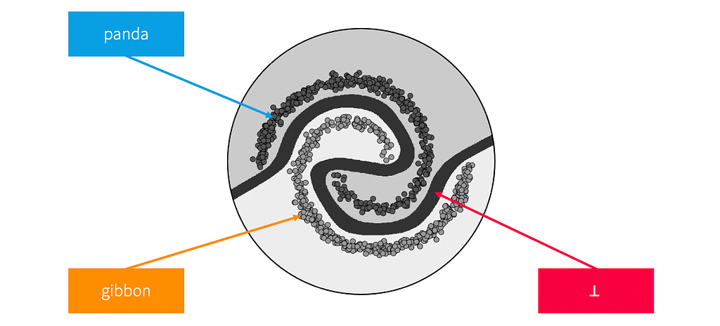
This suggests that we may need to be alright with the network not being locally robust in some places; this doesn’t have to be a problem as long as the network is robust in the places we care about — the regions covered by the data. Therefore, we will think of a model as being robust as long there is a margin of width at least ε on the boundary, separating regions of the input space that are given different labels.
An example of how a robust model might look is shown in the figure below. The margin (shown in black) is essentially a “no man’s land” where the model indicates that points are not locally robust by labeling them with a special label, ⊥ (“bottom,” a mathematical symbol sometimes used to denote null values). Ideally, no “real” data points (e.g., training points, validation points, etc.) lie in this no man’s land.
Constructing Globally-Robust Networks
The key idea behind GloRo Nets is that we want to construct the network in such a way that a margin will automatically be imposed on the boundary.
The output of a neural network classifier is typically what is called a logit vector, containing one dimension (i.e., one logit value) per possible output class. The network makes predictions by selecting the class corresponding to the highest logit value.
When we cross a decision boundary, one logit value will surpass the previous highest logit value. Thus, the decision boundary corresponds to the points where there is a tie for the highest logit output. To create a margin along the boundary, we essentially want to thicken the boundary. We can do this by declaring a tie whenever the two highest logits are too close together; i.e., we will consider the decision a draw unless one logit surpasses the rest by at least δ.
We can let the case of a draw correspond to the ⊥ class. This will create a no-man’s-land region separating the other classes as desired. But it remains to ensure that the width of this region is always at least ε (in the input space). To do this, we will make use of the Lipschitz constant of the network.
Leveraging the Lipschitz Constant
The Lipschitz constant of a function tells us how much the output of the function can change as its input is changed. Intuitively, we can think of it as the maximum slope, or rate-of-change, of the function.
Thus, if the Lipschitz constant of a function is K, then the most the function’s output can change by, if its input changes by a total of ε, is εK. We will use this fact to impose a margin of the correct width on our network’s decision surface.
As a neural network is really just a high-dimensional function, we can also consider the Lipschitz constant of a neural network. For the sake of simplicity, we will consider each logit value as a distinct function with its own Lipschitz constant (this will be sufficient to explain how GloRo Nets work, but the analysis can be tightened by a slightly more complex accounting of the full network’s Lipschitz constant; the appendix of our paper provides these technical details).
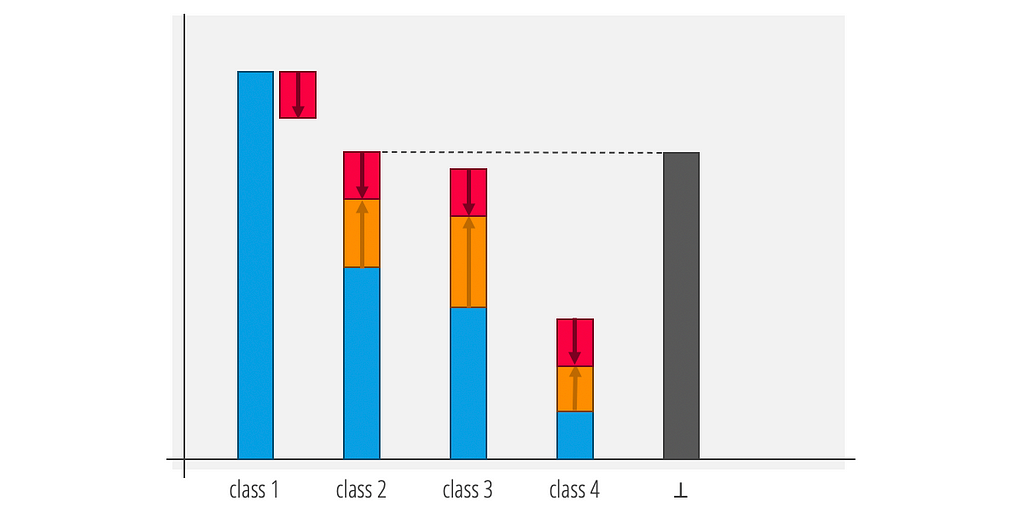
We now return to our intuition from earlier to demonstrate how to construct GloRo Nets, by way of an example.
Suppose we have a network predicting between four classes that produces the logits shown below. If the difference between the logits for class 1 and 2 is sufficiently large, class 2 will not be able to surpass class 1 (and similarly for classes 3 and 4).
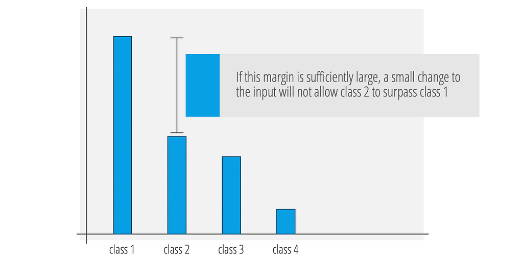
As discussed, the Lipschitz constant tells us how much each logit can move when the input is perturbed within a radius of ε. By considering the amount by which class 1 can decrease, and the amount by which each of the other classes can increase, we can calculate the amount by which each class can gain on the predicted class (class 1). We then insert a new logit value, corresponding to the ⊥ class, which takes its value based on the most competitive class to class 1, after considering how much each class can move.
As a result, we have the following important property: if the ⊥ logit is not the maximum logit at a given point, then we are guaranteed that the model is locally robust at that point. On the other hand, if the ⊥ logit is the maximum logit, the network will predict ⊥ as desired, indicating that the point lies in the margin between classes.
Approximating the Lipschitz Constant
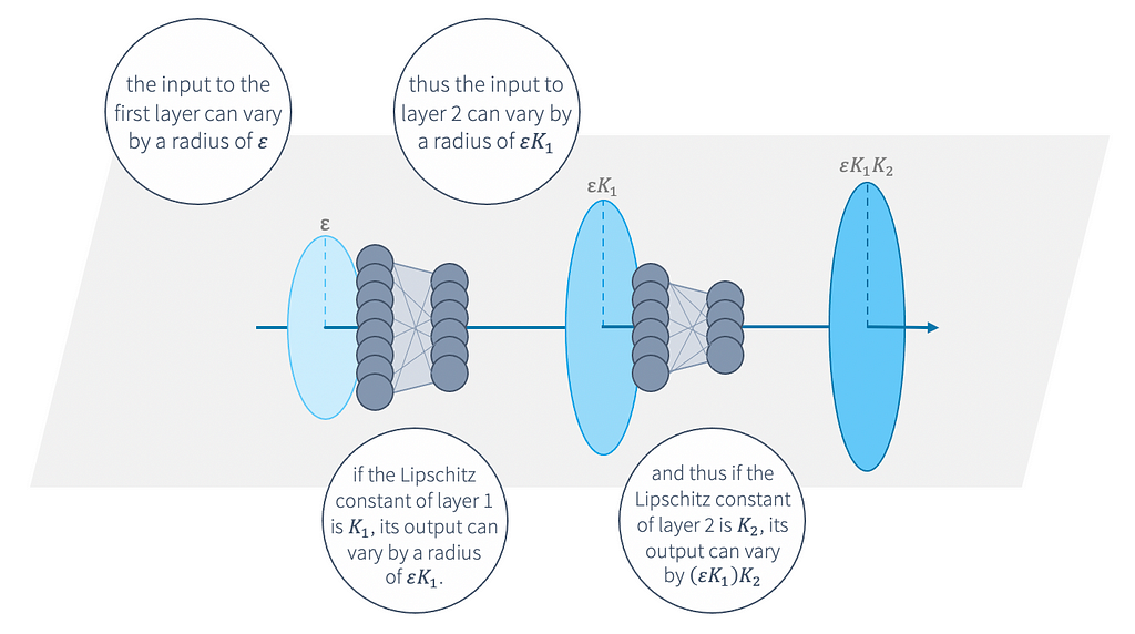
While calculating the exact Lipschitz constant of a neural network is a fundamentally hard problem computationally, we can obtain an upper bound on the Lipschitz constant fairly easily and efficiently by breaking down the computation to consider one layer at a time. Essentially, we can multiply the Lipschitz constant of each of the individual layers together to obtain a bound for the entire network. The figure below gives some intuition as to why this works.
Interestingly, while this bound would usually be very loose on a typical network — that is, it will vastly overestimate the Lipschitz constant — because the bound calculation is incorporated into the learning objective (more on this below), even this naive layer-wise bound ends up fairly tight on GloRo Nets, which are not “typical” networks. This means that using a simple calculation of the Lipschitz constant is actually an effective way to impose a sufficient margin between classes for obtaining provable robustness.
Moreover, after training, the Lipschitz constant will remain fixed. This means that test-time certification does not require any additional computation to compute the Lipschitz bound, making certification essentially free. This is a major advantage compared to other robustness certification approaches, which often require expensive computation to obtain robustness guarantees.
Naturally Capturing a Robust Objective
Conveniently, the way we encode the ⊥ region as an extra class allows us to train GloRo Nets to optimize for provable robustness quite easily. The key to this fact is that in GloRo Nets, robustness is captured by accuracy. Essentially, since ⊥ is never the correct class on our labeled data, by training the network to be accurate (as we usually do), it avoids picking ⊥, which in turn means it avoids being non-robust.
An Illustrative Example with Code
We’ll now take a look at an example of GloRo Nets in action (to follow along interactively, check out this notebook). A library implementing GloRo Nets in TensorFlow/Keras is available here; it can also be installed with pip:
pip install gloro
Using the gloro library, we will see that GloRo Nets are simple to construct and train; and they achieve state-of-the-art performance for certifiably-robust models [1].
We will use the MNIST dataset of hand-written digits as an example. This dataset can be easily obtained through tensorflow-datasets.
import tensorflow as tf
import tensorflow_datasets as tfds
# Load the data.
(train, test), metadata = tfds.load(
    'mnist',
    split=['train', 'test'],
    with_info=True,
    shuffle_files=True,
    as_supervised=True)
# Set up the train and test pipelines.
train = (train
    .map(lambda x,y: (tf.cast(x, 'float32') / 255., y))
    .cache()
    .batch(512))
test = (test
    .map(lambda x,y: (tf.cast(x, 'float32') / 255., y))
    .cache()
    .batch(512))
We begin by defining a simple convolutional network. Constructing a GloRo Net with the gloro library looks pretty much exactly the same as it would in Keras; the only difference is that we instantiate it with the GloroNet class (rather than the default Keras Model class), which requires us to specify a robustness radius, epsilon. While the GloroNet model class is compatible out-of-the-box with any 1-Lipschitz activation function (including ReLU), we find that the MinMax activation, which sorts pairs of neighboring neurons, works best (the reasons why are beyond the scope of this article).
from gloro import GloroNet
from gloro.layers import MinMax
from tensorflow.keras.layers import Conv2D
from tensorflow.keras.layers import Dense
from tensorflow.keras.layers import Flatten
from tensorflow.keras.layers import Input
x = Input((28, 28, 1))
z = Conv2D(
    16, 4,
    strides=2,
    padding='same',
    kernel_initializer='orthogonal')(x)
z = MinMax()(z)
z = Conv2D(
    32, 4,
    strides=2,
    padding='same',
    kernel_initializer='orthogonal')(z)
z = MinMax()(z)
z = Flatten()(z)
z = Dense(100, kernel_initializer='orthogonal')(z)
z = MinMax()(z)
y = Dense(10, kernel_initializer='orthogonal')(z)
g = GloroNet(x, y, epsilon=0.3)
We can then compile the model. There are a few choices for GloRo-Net-compatible loss functions, including standard categorical cross-entropy, but we typically find that Trades loss (found in gloro.training.losses) works best (the details for the different loss functions are not in the scope of this article).
We also find the clean_acc and vra metrics to be useful for tracking progress. Clean accuracy is the accuracy the model achieves when the margin is ignored (i.e., if we don’t care about robustness). VRA, or verified-robust accuracy is the fraction of points that are both correctly classified and certified as locally robust; this is the typical success metric for robust models.
# Use TRADES loss with crossentropy and a TRADES
# parameter of 1.2.
g.compile(
    loss='sparse_trades_ce.1.2',
    optimizer='adam',
    metrics=['clean_acc', 'vra'])
Finally, we are ready to fit our model to our data. The gloro library contains a number of useful callbacks to define a schedule for the various hyper-parameters; these are helpful for getting the best performance out of training. For example, we find that slowly raising the robustness radius over the course of training results in a better outcome.
from gloro.training.callbacks import EpsilonScheduler
from gloro.training.callbacks import LrScheduler
g.fit(
    train,
    epochs=50,
    validation_data=test,
    callbacks=[
        # Scale epsilon from 10% of our target value
        # (0.03) to 100% of our target value (0.3)
        # half-way through training.
        EpsilonScheduler('[0.1]-log-[50%:1.0]'),
        # Decay the learning rate linearly to 0 half-
        # way through training.
        LrScheduler('[1.0]-[50%:1.0]-[0.0]'),
    ])
And that’s it! This results in the following clean accuracy and VRA:
test clean_acc: 99.1%
test vra:       95.8%
Summary
GloRo Nets provide an elegant and effective way to guard against small-norm adversarial examples by automatically inducing an ε-margin into the construction of the network. Because robustness certification is naturally incorporated into the network’s output, GloRo Nets can be easily optimized for verified-robust accuracy, and can perform essentially-free certification at test time. Moreover, because the Lipschitz bounds used to certify the network are also incorporated into the network, GloRo Nets can achieve state-of-the-art VRA using simple, efficiently-computable upper bounds for the Lipchitz constant.
References
- Leino et al. “Globally-Robust Neural Networks.” ICML 2021. ArXiv
- Goodfellow et al. “Explaining and Harnessing Adversarial Examples.” ICLR 2015. ArXiv
Training Provably-Robust Neural Networks was originally published in Towards Data Science on Medium, where people are continuing the conversation by highlighting and responding to this story.
from Towards Data Science - Medium https://ift.tt/3HkLYmi
via RiYo Analytics


No comments