https://ift.tt/3jZIOdS ARTIFICIAL INTELLIGENCE How to remove extra noise in your audio data Mood — Photo by Francesco De Tommaso on Un...
ARTIFICIAL INTELLIGENCE
How to remove extra noise in your audio data
Upon first entering the data science field through the Flatiron School, I had my eyes set on the prospect of combining my ongoing training with my background in music. The final requirement of the course was the capstone project. The objective was to solve a problem of interest with the culmination of our newly acquired skills. I felt like this was the golden opportunity to begin understanding the interrelatedness of music and machine learning.
My instructor and I discussed the scope of the project in many of our meetings. At first I wanted to create a generative model for music synthesis. I then became interested in the musicality of non-human animals, particularly whale songs. Together we looked for data and discovered not whales, but birds: the BirdCLEF 2021 bird call identification dataset. This is a niche yet open-ended collection of audio data. Upon digging deeper into the data, I learned that the implications are far from easily pigeonholed, yet have avenues of great specificity. Audio data can add another dimension to ornithological research and the implementation of conservation efforts for endangered species. It also allows recreational birdwatchers to more easily identify birds they are not able to otherwise see. Sonically, I see great opportunities for studying the musicality of bird vocalizations and using the identified bird as a source of artistic inspiration.

I want to share a neat thing I used (thanks to the great help of Seth Adams) to help preprocess the audio data: the signal envelope. The envelope outlines the highest and lowest points (dB) of an audio signal. This is one part of the larger preprocessing objective: to quantify the physical properties of an audio signal. There are several measurements, such as the sample rate (n data points per second), amplitude (dB), frequency (Hz). The envelope incorporates these elements and is a tool that becomes highly useful, if not necessary, for cleaning audio data, particularly for environmental recordings. The purpose of gathering the extreme values of an audio signal is to reduce environmental noise in the recording so the model can focus on the values of the vocalization during training.
I mainly used these libraries for the task: Pandas, NumPy, Librosa, and Matplotlib. I found Librosa to be really neat. It’s widely used for analyzing audio data and, in this example, performs several key functions. In sum, the pipeline used to train my model on audio data includes (1) loading the raw audio file; (2) converting into a waveform; (3) transforming the waveform into a Mel Spectrogram. I’ll mainly focus on the first two steps.
Below is the code for the main envelope function, which takes in three arguments: audio signal, sample rate, and threshold. Under the hood, it converts a signal into a Pandas series and takes the absolute value of all of its data points. From here, a rolling window is used to take the average of every window of sample_rate(Hz)/10 points. A for loop is used to iterate through the Pandas series of mean signals. If any of the new data points are above the threshold (dB), which you set, it will be appended to a NumPy array called mask (I used this name to remain consistent with Seth’s work). Any data points below the threshold will not be included in the array.
Function without signal envelope:
"""
    Inputs audio data in the form of a numpy array. Converts to pandas series
    to find the rolling average and apply the absolute value to the signal at all points.

    Additionally takes in the sample rate and threshold (amplitude). Data below the threshold
    will be filtered out. This is useful for filtering out environmental noise from recordings.
    """
    mask = []
    signal = pd.Series(signal).apply(np.abs) # Convert to series to find rolling average and apply absolute value to the signal at all points.
    signal_mean = signal.rolling(window = int(rate/10), min_periods = 1, center = True).mean() # Take the rolling average of the series within our specified window.

    for mean in signal_mean:
        if mean > threshold:
            mask.append(True)
        else:
            mask.append(False)
    return np.array(mask)
You may be wondering where the array of averaged data points fits into the rest of the preprocessing steps? Introducing the Fast Fourier Transform (FFT), a significant function for preprocessing audio. The FFT converts a signal of one domain to another domain. For example, if we look below at the audio waveform (pardon the unlabeled axes), it is in the time domain, meaning the amplitude (dB) of the signal is measured over time. The FFT will convert the signal into the frequency domain, which will display the concentration of spectral frequencies of a vocalization; this is known as a periodogram. Though they are two separate function, the signal envelope and FFT ideally work in tandem to prepare the conversion of a waveform image into a Mel Spectrogram.
Function to calculate FFT:
"""
    Performs fast fourier transform, converting time series data into frequency domain.
    """
    n = len(y)
    freq = np.fft.rfftfreq(n, d=(1/rate))
    Y = abs(np.fft.rfft(y)/n)
    return (Y, freq)
I’ve included two sets of the code with these functions in use. Both of which are the same except that the latter includes the envelope function shown earlier. Two blank dictionaries are defined, one for the original signal quantities and one for the FFT signal quantities. The for loop iterates through a list of bird classes, where it will match the class to the label in the metadata dataframe. Afterwards, the audio directories are searched via Librosa’s load function to match the label in the audio file directory and load it as a mono signal at a sample rate set above (16kHz). The signal is then labeled according to the bird class and subsequently undergoes an FFT at a sample rate of 16kHz. Both the original signal and FFT signals are added to the dictionaries with their labels. Let’s look below.
Function with signal envelope:
try:
    sig = {}
    fft = {}

    for c in classes:
        audio_file = TRAIN[TRAIN['primary_label'] == c].iloc[0,9]
        signal, rate = librosa.load(MAIN_DIR+'train_short_audio/'+c+'/'+audio_file, coefs.sr, mono=True)
        sig[c] = signal
        fft[c] = fft_calc(sig[c], 16000) #included fast fourier transform
plot_signals(sig)
except IndexError:
    pass
The envelope function is called after loading the data and before the FFT. The new signal is redefined as what I call the “enveloped” signal; this is added to the sig_new dictionary. The new signal then undergoes an FFT.
try:
    sig_new = {}
    fft_new = {}

    # Clean displayed audio from above.
    for c in classes:
        audio_file = TRAIN[TRAIN['primary_label'] == c].iloc[0,9]
        signal, rate = librosa.load(MAIN_DIR+'train_short_audio/'+c+'/'+audio_file, sr=coefs.sr, mono=True)
        mask = envelope(signal, rate, 0.009) #(array, sample_rate, dB threshold)
        signal = signal[mask]
        sig_new[c] = signal
        fft_new[c] = fft_calc(sig_new[c], 16000)
plot_signals(sig_new)

except IndexError:
    pass
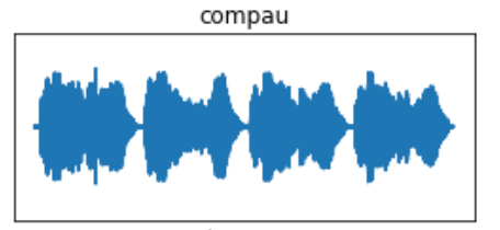
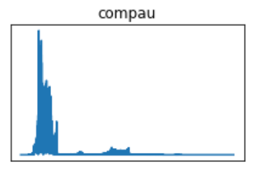
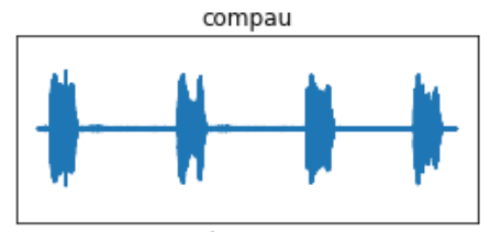
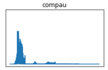
I’ve used one species, the Common Pauraque, as an example. The pre-FFT images show what appears to be more robust waveforms, but that is a result of eliminating the data below the dB threshold of 0.009. The same principle goes for the FFT periodograms, in which the eliminated data will display greater concentrations of the frequencies in the vocalization.
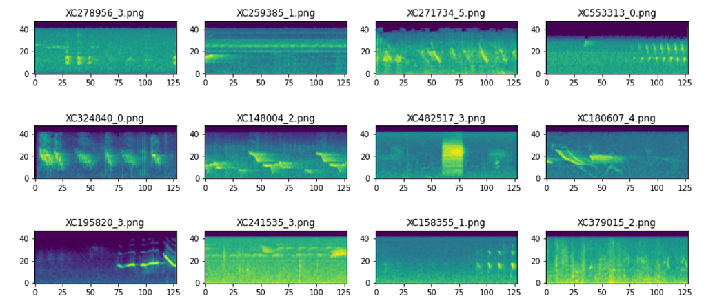
To bring it all together, here are 12 samples of Mel Spectrograms after the signal envelope and FFT have been applied to all signals. The brighter colors signify greater concentrations of frequencies (kHz). Now, the audio classification task has become an image classification task.
It is important to note that this function was used on 27 bird species, each of which contain hundreds of recordings of varying fidelity. The magnitude of its effect inherently varies from recording to recording. While still a useful preprocessing step, it is difficult to determine consistency and if all desired information will be preserved after a formulaic data slice. Nonetheless, I highly recommend audio machine learning practitioners incorporate this function to bring themselves one step closer to working with more organized data.
Please feel free to check out the project here, to ask me questions for clarity, or to suggest ways of moving this forward into its best possible version. Thanks so much!
References:
- Seth Adams
- Stefan Kahl
- Ayush Thakur
- DrCapa
- Andrey Shtrauss
- Valerio Velardo
- Francois Lemarchand
- Adam Sabra
Preprocess Audio Data with the Signal Envelope was originally published in Towards Data Science on Medium, where people are continuing the conversation by highlighting and responding to this story.
from Towards Data Science - Medium https://ift.tt/31jzbjD
via RiYo Analytics


No comments