https://ift.tt/31id25u How to connect the Multi-Armed Bandit problem to a clustering algorithm Photo by Kristaps Grundsteins on Unsplas...
How to connect the Multi-Armed Bandit problem to a clustering algorithm

Presentation
BanditPAM, with a less evocative name than its famous brother KMeans, is a clustering algorithm. It belongs to the KMedoids family of algorithms and was presented at the NeurIPS conference in 2020 (link to the paper).
Before diving into the details, let’s explain the differences with KMeans.
The main distinction comes from the “Means” and “Medoids” but the structure is the same.
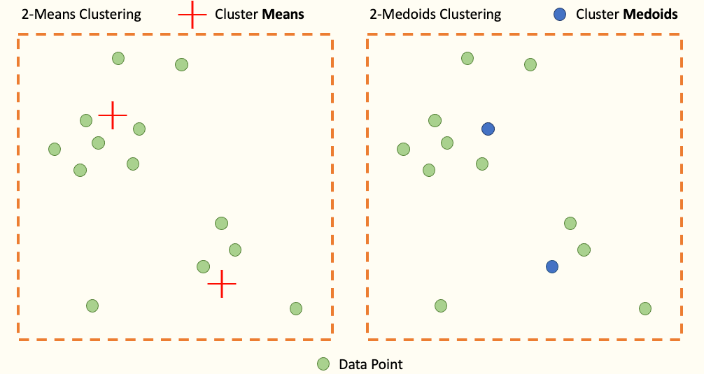
As shown in the picture, KMeans positions the center of its cluster (i.e. its centroid) by minimizing the Euclidean distance to each point in the same cluster. Thus, it is the mean (KMeans) of the points in its cluster. On its side, the KMedoids positions the center of its cluster on a point of the dataset minimizing the distance with the other points of the same cluster. We call these centers Medoids
In other words, the center of each KMedoids cluster is necessarily a point existing in the dataset (contrary to K-Means)
So What?
In some problems, considering medoids allows a better understanding and explicability of the result as well as an improvement of the clustering for so-called “structured” objects (often data tables)
Why Now?
KMeans has always dominated the subject of clustering algorithms because of its simplicity of operation but especially because of its low complexity. Indeed, the complexity of KMeans is often linear according to the number of points in the dataset n, to the number of clusters k and, to the number of dimensions d. It’s a different story for KMedoids since even the state of the art called PAM — for Partitioning Around Medoids — has quadratic complexity.
It is on this precise point that the research paper made its reputation by implementing BanditPAM, an improvement of PAM from a quadratic complexity to a “quasi-linear” complexity according to the research paper (precisely in O[nlog(n)])
BanditPAM is based on 2 algorithms:
- PAM — Partitioning Around Medoids
- Multi-Armed Bandit
Partitioning Around Medoids (or PAM)
1. Presentation
The objective of PAM, like all clustering algorithms, is to obtain the best quality of clustering performed.
By noting d( . , . ) the distance metric (Euclidean distance, cosine similarity, …) and M the set of medoids, this quality is obtained through this cost function:

In other words, the objective of PAM is to find the set of KMedoids allowing to minimize the distance of the points to its closest medoid.
This algorithm is based on 2 steps comparable to KMeans.
2. BUILD (the initialization phase)
During this phase, PAM initializes its k medoids according to a specific rule.
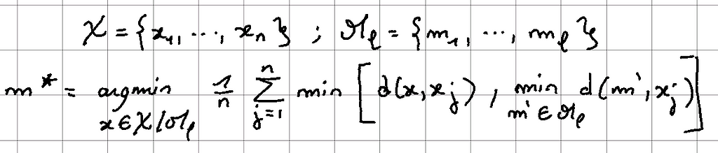
With N points and L medoids already initialized, we find the next medoid m* according to the following relation:
Let us illustrate this step through an example:
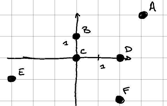
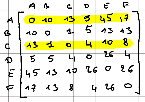
Let us consider 6 points (A, B, C, D, E, F), and let us try to define the 2 medoids according to the BUILD step defined above.
For this example, we define the distance between 2 points as the square of the Euclidean distance.
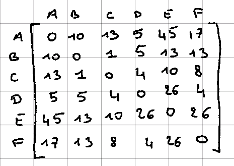
Thus, we obtain this distance matrix where all further calculations will be referred to this matrix
1.a Define the first medoid
Since it is the first medoid that we wish to calculate, we obtain the following relation:
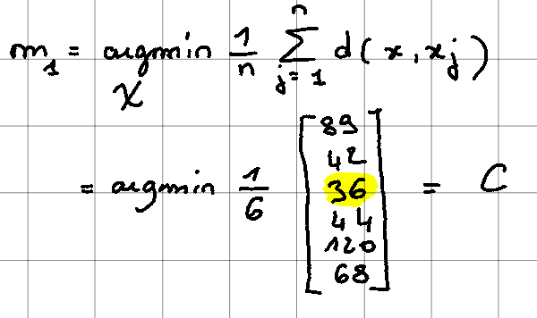
Here we notice that the relationship is different since no minimum is present. This is because at this stage the set M is empty and therefore the second minimum is not defined.
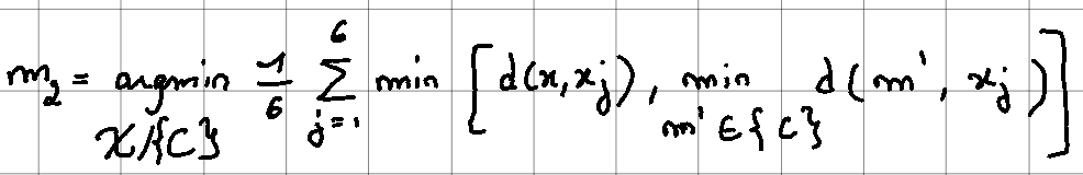
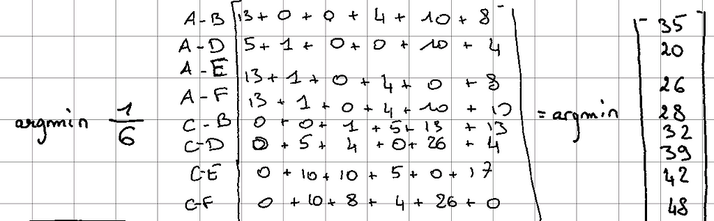
1.b Defining the second medoid
This step can be more complex to understand as we are using the whole relationship:
Taking the matrix again, we have the following result:
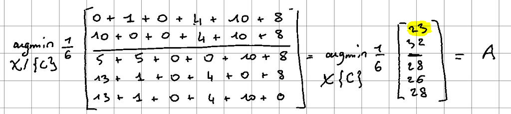
Since we have set ourselves to 2 medoids, the initialization step is over. A and C have been chosen and the cost function is:

We have defined the 2 medoids as expected, so the initialization is finished. Let’s move on to the SWAP phase — the optimization phase.
2. SWAP (the optimization phase)
Again intending to minimize the objective function, this step tries to swap some medoids with non-medoids. In other words, a medoid becomes a “normal” point and a “normal” point becomes a medoid. A “normal” point is a point that is not a medoid. Among all possible pairs, the selected pair follows the following relationship:
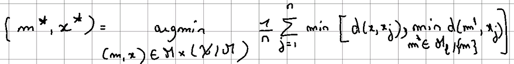
Once m* and x* are found, x* becomes a medoid, and m* becomes a “normal” point again.
As a reminder, we have this distance matrix but now with A and C, the 2 initialized medoids.
By applying the SWAP relation above, we have:
In this case, the minimum is the link between medoid A and point D.
A becomes a non-medoid point and D a medoid if and only if the cost function with A and D as medoid is lower than the one calculated with A and C.
But here:
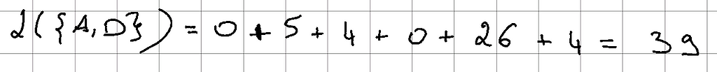
As 39 > 23, A and D are not inverted and convergence is assumed. The algorithm stops.
If the value is less than 23, we would have reversed A & D and the SWAP process would have repeated itself until convergence (i.e. the cost function no longer decreases)
3. The problem
In a more general example with n points and k medoids, the complexity is quadratic.
Why is this so?
In the BUILD step, for each medoid, we are interested in each of the n points. For each point, a summation over n is performed (see BUILD relation). Thus, the complexity is n*n and therefore quadratic. In reality, since there are k medoids, the complexity is O(k*n*n).
The same reasoning works for SWAP.
The general complexity of the algorithm is therefore quadratic.
To overcome this problem, BanditPAM uses the Multi-Armed Bandit algorithm to change the complexity from quadratic to n*log(n).
Multi-Armed Bandit (or MAB)
The Multi-Armed Bandit is a problem that involves the dilemma: exploration vs. exploitation. A brief explanation of this dilemma is necessary.
1. Context of the problem
Let’s imagine Pierre, a young worker living in Paris with his parents for 1 year. Unfortunately, Pierre does not excel in the art of cooking and is used to eating out whenever he is home alone. When the time comes to choose, Peter is always faced with the same dilemma: “Do I go back to one of the restaurants which have already satisfied me, or do I risk trying a new restaurant (for better or for worth)?
This problem illustrates the Multi-Armed Bandit:
Several actions are possible (restaurants) and each action provides a reward (satisfaction with the food, the style, the service …) which can be both positive and negative. However, the reward is not constant for the same action, i.e. if Peter goes to a restaurant at 2 different times, he may love it one time and hate it the other.
2. Possible strategies
So what is the best strategy to adopt?
- Continue to perform the same action that gives the best reward?
- Take the risk of constantly choosing new actions in the hope that they will provide a better reward than the previous ones?
The first strategy is called exploitation. One exploits a single action without knowing the rewards of the other actions. If Peter follows this strategy, he chooses his favorite restaurant (i.e. with the best reward) and sticks to it without ever eating anywhere else…
The other strategy is called exploration. This consists of always exploring the other actions to acquire as much information as possible to finally choose the best action.
3. Existing algorithms
Fortunately, the subject has already existing solutions.
The ε-greedy algorithm consists in exploring — with a probability ε — the possible actions. If this is the case, the exploration is done randomly. Otherwise, the best action is chosen.
If Peter, when choosing his restaurant, follows this “ε-greedy” strategy, he has a probability ε (e.g. 0.05 or 5%) of randomly choosing a new restaurant. He, therefore, has a 95% chance of returning to his favorite restaurant.
With Multi-Armed Bandit, this exploration is not random but considered smarter. In particular, at each step, the action chosen is dictated by an algorithm called UCB for Upper Confidence Bounds
(Note that other algorithms than UCB exist but UCB is mentioned in the research paper)
4. Overview of UCB
The problem with random exploration is that it is possible to run into bad actions that you have already run into before.
As a reminder, the reward is not a fixed value per restaurant but depends on the given moment. By including the notion of rating, Peter may go to eat in a restaurant that he has already appreciated to the extent of 4 stars out of 5 but his second attempt 1 month later ended with a 1 star out of 5. This type of restaurant is therefore highly uncertain, unlike other restaurants where each visit by Pierre ended with approximately the same “score” (= reward).
UCB’s algorithm is to prefers very uncertain actions. Otherwise, actions that have a consistent reward history are avoided. The aim is to favor the exploration of actions that have a greater potential to have the optimal reward.
By analogy with Peter’s case, if he follows the UCB strategy, he will choose one of the restaurants where his reviews have been very different between his different visits. Thus, if he has already been to a restaurant four times and the ratings have always been relatively the same, it is very unlikely that the fifth time around, this restaurant will become the best.
When choosing the t-th restaurant, the choice respects the following relation:
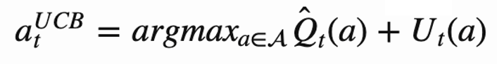
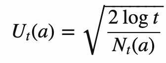
In other words, the action chosen is the one that maximizes the average of the reward history of action and the second term U.
Very simply, the more the same action is performed, the more Nt(a) increases and therefore Ut(a) decreases. Action “a” is less likely to be chosen.
In Peter’s case, the more he chooses the same restaurant, the higher Nt(a) is and the more the Q + U term decreases and the less likely the action is to be chosen.
Bandit + PAM = BanditPAM
The presence of the Multi-Armed Bandit in the PAM algorithm allows us to move from a computational problem to a statistical problem.
Indeed, the MAB can be inserted in the SWAP and BUILD steps quite easily.
For the SWAP step, the analogy is the following:
- Simply consider a medoid/non-medoid pair as a possible action and the associated reward is the value of the cost function to be minimized. The closer the cost function is to 0, the higher the reward.
Thus, PAM avoids computing all possible pairs (n*(n-k)) but selects the best pair via the PAM algorithm. As a result, the complexity becomes n*log(n).
For the BUILD step, the analogy is the following:
- Each possible candidate is an action and the reward is the computation of the cost function as for the SWAP step but only for a random sample of the data. This allows that, for the same candidate tested, the value of the reward is different following the PAM algorithm.
The use of BanditPAM is implemented in python via Python.
The GitHub with examples: https://github.com/ThrunGroup/BanditPAM/
Conclusion
This introduction to BanditPAM has allowed us to look independently at two algorithms. The addition of a statistical model (PAM) in the KMedoids algorithm improves the complexity while keeping a relatively good clustering quality.
More details are provided on how to include the Multi-Armed Bandit within the PAM in the research paper. This handling is not so obvious and I invite all curious to look at the original paper.
Thank you for reading my first article, please feel free to support, comment, and share if you liked it.
Source
- BanditPAM: https://paperswithcode.com/paper/bandit-pam-almost-linear-time-k-medoids
- Multi-Armed Bandit: https://lilianweng.github.io/lil-log/2018/01/23/the-multi-armed-bandit-problem-and-its-solutions.html
Introduction to BanditPAM was originally published in Towards Data Science on Medium, where people are continuing the conversation by highlighting and responding to this story.
from Towards Data Science - Medium https://ift.tt/31a1OQg
via RiYo Analytics


ليست هناك تعليقات