https://ift.tt/3ljcZNP Learning chess by combining AlphaGo and Transformers Hi everyone, this will be the second instalment in my tutorial...
Learning chess by combining AlphaGo and Transformers
Hi everyone, this will be the second instalment in my tutorial series for building a chess engine. This lesson will focus on building an AI agent that we can play. This lesson is going to be more technical than part 1, so please bear with me. I try to supply both equations and diagrams to help make things a little easier.
Now that we have finished building our chess game, we can begin designing an AI that plays it. Chess AI’s have been successful for many years now, from deep blue to stockfish. However, there is a new program that has become state of the art using deep learning. AlphaZero is a reinforcement learning agent by DeepMind that has achieved superhuman level results in numerous games (Chess, Shogi, GO).
Because of this success, we will build off of AlphaZero and use its powerful idea of guiding the Monte Carlo Tree Search (MCTS) algorithm with a deep learning model. Instead of using a Convolution Neural Net (CNN) like the one used in their paper, we will use a Transformer. Transformers have found great success recently in many fields such as Natural Language Processing (NLP) and Computer Vision (CV). Because of this, it seems fitting that we could try to use one here.
Monte Carlo Tree Search (MCTS)
In all games, there are a series of actions. In game theory, it is common to represent these actions in a game tree.
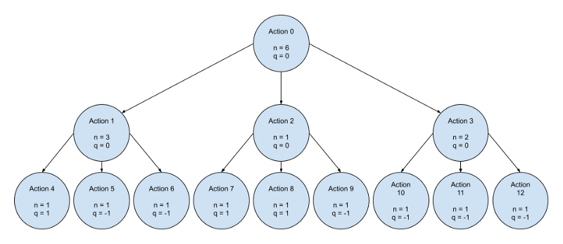
In simple games, a game tree is small and can be brute-force searched. With small game trees, we can use greedy algorithms like the “MiniMax” search algorithm. Most games aren’t simple though this causes brute-force methods to be deemed infeasible within modern computational limits. Because of this, other search algorithms like MCTS prove to be more beneficial.
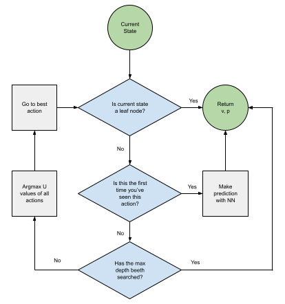
MCTS first checks if the current state is a leaf node (end of the game) or not. If the current state is a leaf node, the search algorithm returns the results of the game.

- sw = white win (0 or 1)
- st = tie game (0 or 1)
- sb = black win (0 or 1)
If the action is not a leaf node and this is the first time seeing it, the Neural Net (NN) is used to determine the value (v) of the current state and probability (p) of all possible actions. The current states node reward value is the newly predicted value. The probability of all possible valid actions is updated using the predicted probability distribution. We return the value (v) and probability (p) for the previous nodes to be updated.
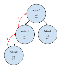
If we have seen the current state before, we recursively search the action with the highest UCB.
UCB is a powerful formula that tries to balance exploitation and exploration. The first half of the equation exploits the AI’s game knowledge. The second half enhances exploration by multiplying a hyperparameter(c) by the probability (p).
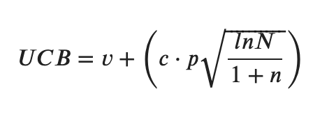
- v = end game value
- c = exploration hyper parameter [0–1]
- p = action probability
- N = parent node visits
- n = action node visits
When searching the game tree, if the current depth is equal to the max allowable depth, the value (v) and probability (p) at the current depth is returned for the previous nodes to be updated.
Model Architecture
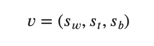
With this knowledge of MCTS, let us talk about our model. Our model will get the game state as an input and returns the expected game outcome along with the action probability distribution.
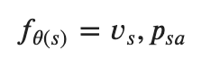
- vs = probability distribution of game results based on the current state
- psa = probability distribution for all actions of the current state
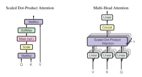
The main component of our model is a transformer. Transformers have been talked about a lot recently and have been seen increasingly in state-of-the-art systems. Transformers are very effective through their use of the attention mechanism (multi-head scaled dot-product attention).
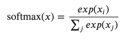
Attention is a powerful equation that allows the model to learn which things are important and deserve more focus. It does this by taking the scaled dot product of a query and a key to determining the similarity of the two. Dot product determines the similarity by finding the angle between the inputs. Softmax then scales the result between 0–1. The dot product is taken of the resultant and value to determine the similarity of the two. This second dot product has another useful feature and helps the output keep its initial shape.
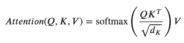
- Q = Q(E) = query (vector/matrix)
- K = K(E) = key (vector/matrix)
- V = V(E) = value (vector/matrix)
- E = embeddings
Multi-Head attention breaks the input into multiple heads, processing different chunks in parallel. It’s thought that multi-head attention gets its superior strength through the creation of different subspaces. The results of each head are then concatenated together and passed to a linear layer that maps the input back to its original dimension.
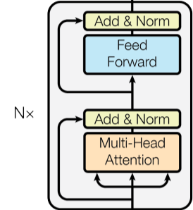
Vanilla transformers have a simple encoder and decoder architecture.
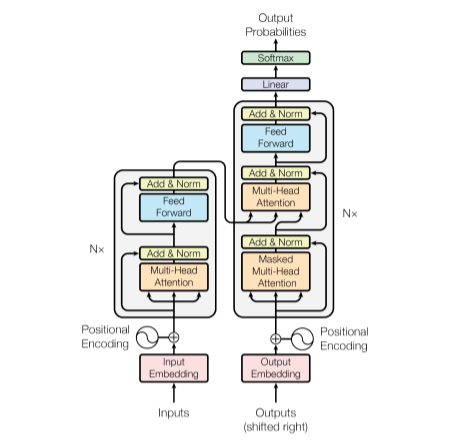
However, we aren’t going to use this architecture and are going to use a decoder-only transformer. A decoder-only transformer looks like the encoder in the transformer architecture diagram from the “Attention is All You Need” paper. When you compare the encoder block and the decoder block above, you’ll find there is only one difference, the lack of an encoder-decoder attention layer in the encoder. This encoder-decoder attention layer isn’t needed in a decoder-only transformer since there is no encoder, meaning we can utilize the encoder block to create a decoder-only model.
After the transformer block, the rest of our model is quite simple. We add a linear layer to map the output of our Transformer layers to our needed dimension (1D).
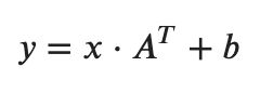
- x = input (vector/matrix)
- A = layer weights (vector/matrix)
- b = layer bias (vector/matrix)
The model then branches off into two parallel linear layers (v, p). These linear layers are here to map each output to its desired size. One of these layers will be the size of the game result (v), while the other is the size of the action state (p). After the linear layers, a softmax is applied to both outputs independently to convert their results to a probability distribution.
- x = input (vector/matrix)
Input Encoding
Now that we know about the model architecture we are using, we should probably talk about the input data. The model will receive the state of the game as input but is unable to process this directly. For the state of the game to be processed, it will need to be encoded. For this, we will use embeddings through a tokenized approach. These embeddings are unique vectors that will represent every piece. Embeddings allow our model to gain a strong representation of the correlation between each game piece.

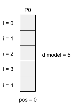
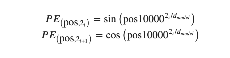
Transformer models process input sequences in parallel resulting in them discarding positional information. Luckily we can add a positional encoding to our input to help restore this additional information. Positional encoding allows the model to extract extra information from each embedding based on its position in the input sequence. This extra information represents the relationship between each piece and its location on the game board.
Output Encoding
With this understanding of the input, let us talk about the output. The model will have two output values. One represents the probability distribution of the possible outcomes (reward), and the other represents the probability distribution of actions (policy).
In our chess game, the possible outcomes are white wins, a tie game and black wins. Since these outcomes are on the nominal scale, we know this is a classification problem. One-hot encodings are popular among classification problems since each bit can represent a different outcome. To determine the index of the most probable outcome of the game, we can take the argmax of the output. From this, we now know the most probable outcome of the game and the confidence in that prediction.
- sw = white win (0 or 1)
- st = tie game (0 or 1)
- sb = black win (0 or 1)
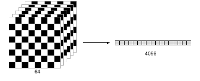
In chess, the pieces are constantly moving. This movement makes it difficult to map our valid actions back to the current state. To mitigate this problem, we will think of the actions as which square moves to which square. Here we effectively simplify the decoding process as the squares on the board stay constant the entire game. We can then represent this with a flattened 64x64 matrix. Flattening the matrix is necessary since this is a classification problem again as our actions are nominal. Because of this, we will want to use one-hot encoding to represent our actions space. To determine the index of the most probable action taken, we filter out the invalid actions and take the argmax of the output. From this, we now know the most probable valid action and the confidence in that prediction.
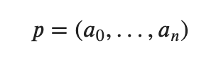
- a= action probability (0–1)
Training Model
Similar to AlphaZero our model learns entirely through self-play. In our version, we add an evolutionary aspect to self-play by having two models (active, new) compete against each other in a round-robin series. In our round-robin series, the new model trains after every game. If the new model is the winner of the round-robin, it becomes the active model. With this, we minimize potential diminishing returns caused by self-play.
The model is trained on the results of every game to minimize the loss in both the predicted game outcome and the predicted action(reward & policy network). For this, the model uses the Binary Cross Entropy of both outputs (BCE). BCE is the loss function because of how well it works with multivariable classification problems.
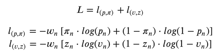
- p = action probability distribution
- pi = one-hot encoding of action taken
- v = game results probability distribution
- z = one-hot encoding of game results
Thanks
And there you have it we have successfully created a chess AI. This AI will start with no knowledge and learn the game of chess. The more training games it plays, the better it will perform. I hope you enjoyed reading part 2 of this series. You can check a full version of the code on my GitHub here. You can also see part 1 of the series here.
References
- https://en.wikipedia.org/wiki/Deep_Blue_(chess_computer)
- https://en.wikipedia.org/wiki/Stockfish_(chess)
- https://deepmind.com/blog/article/alphazero-shedding-new-light-grand-games-chess-shogi-and-go
- https://deepmind.com/
- https://en.wikipedia.org/wiki/Monte_Carlo_tree_search
- https://en.wikipedia.org/wiki/Convolutional_neural_network
- https://en.wikipedia.org/wiki/Minimax
- https://jalammar.github.io/illustrated-transformer/
- https://kazemnejad.com/blog/transformer_architecture_positional_encoding/
- https://en.wikipedia.org/wiki/One-hot
- https://arxiv.org/abs/1706.03762
Building a Chess Engine: Part 2 was originally published in Towards Data Science on Medium, where people are continuing the conversation by highlighting and responding to this story.
from Towards Data Science - Medium https://ift.tt/3cZRiO2
via RiYo Analytics


ليست هناك تعليقات