https://ift.tt/3DRpPds Reduced Regression Models for Time Series Forecasting Photo by Serg Antonov on Unsplash 📚 Introduction Have ...
Reduced Regression Models for Time Series Forecasting

📚 Introduction
Have you ever looked at a model’s hyperparameters and wondered what impact they have on the model’s performance? Well, you are not alone. While some of the impact can be derived intuitively, in other cases, the results are counter intuitive. This is exacerbated by the fact that these hyperparameters do not work alone (univariate) but in conjunction with each other (multivariate). Understanding the impact of hyperparameters on the model’s performance becomes even more important when deciding the search space for a grid search. Choosing the wrong search space can lead to wasted wall clock time while not improving the model performance.
In this article, we will see how we can use Pycaret in conjunction with MLFlow to gain a better understanding of model hyperparameters. This will help us in choosing a good search space while performing grid search.
📖 Suggested Previous Reads
In this article, we will use PyCaret’s Time Series module as an example to explore this concept. Specifically, we will look at reduced regression models for forecasting. If you are not familiar with these models, I would recommend this short read.
👉 Reduced Regression Models for Time Series Forecasting
Also, if you are not familiar with how PyCaret and MLFlow work together, this is a short read that would be helpful.
👉 Time Series Experimental Logging with MLFlow
1️⃣ Reduced Regression Model Hyperparameters
Reduced regression models come with several hyperparameters, but a couple of important ones are sp and window_length. In the “previous read” above, it is suggested that the data be de-seasonalized before passing to the regressor for modeling. sp represents the seasonal period to be used for de-seasonalizing the data. In addition, the modeler needs to decide how many previous lags to feed into the regression model during the training process. This is controlled by the window_length hyperparameter.
sp : int, optional
Seasonality period used to deseasonalize, by default 1
window_length : int, optional
Window Length used for the Reduced Forecaster, by default 10
2️⃣ Hyperparameter Intuition
Many datasets exhibit seasonal patterns. This means that the value at any given point in time will closely follow the data from one or more seasons back (determined by the seasonal period or sp). Hence, it might be intuitive to keep sp fixed to the seasonal period (which can be derived from the ACF plots for example). Similarly, one may want to pass at least one season’s worth of data to the regressor for modeling the auto-regressive properties. Hence, our intuition might tell us to keep window_length to be equal to the seasonal period as well.
3️⃣ Experimentation with PyCaret
Now, let’s take a dataset and see what impact these hyperparameters have. We will use the classical “airline” dataset for this exercise. NOTE: A Jupyter notebook for this article is provided at the end for reference.

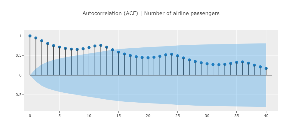
This datasets exhibits a seasonal pattern of 12 month which is indicated by the peaking in the ACF at multiple of 12 (12, 24, 36, etc.)
Experimenting with Window Length
Let’s create a pycaret experiment where we change the window_length and examine the impact it has on the model performance. We will enable MLflow logging in the setup.
exp.setup(
    data=y, fh=12, session_id=42,
    log_experiment=True,
    experiment_name="my_exp_hyper_window",
    log_plots=True
)
#### Create models with varying window lengths ----
for window_length in np.arange(1, 25):
    exp.create_model("lr_cds_dt", window_length=window_length)
The results of this experiment can now be visualized in MLflow. MLflow provides a very handy feature to compare multiple runs of an experiment. We can use this feature to see the impact of window_length.
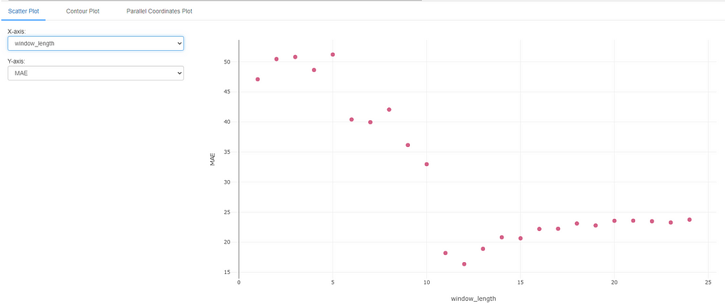
The results match with our intuition that including at least 12 points in the window provides the best performance. Anything less than 11 points tends to degrade the performance since we have not included the data from one season back. Anything more than 12 data points results in a fairly stable result close to the optimal metric value.
Experimenting with Seasonal Period
Next, let’s repeat the same for sp.
#### Setup experiment with MLFlow logging ----
exp.setup(
    data=y, fh=12, session_id=42,
    log_experiment=True,
    experiment_name="my_exp_hyper_sp",
    log_plots=True
)
#### Create a model with varying seasonal periods ----
for sp in np.arange(1, 25):
    model = exp.create_model("lr_cds_dt", sp=sp)
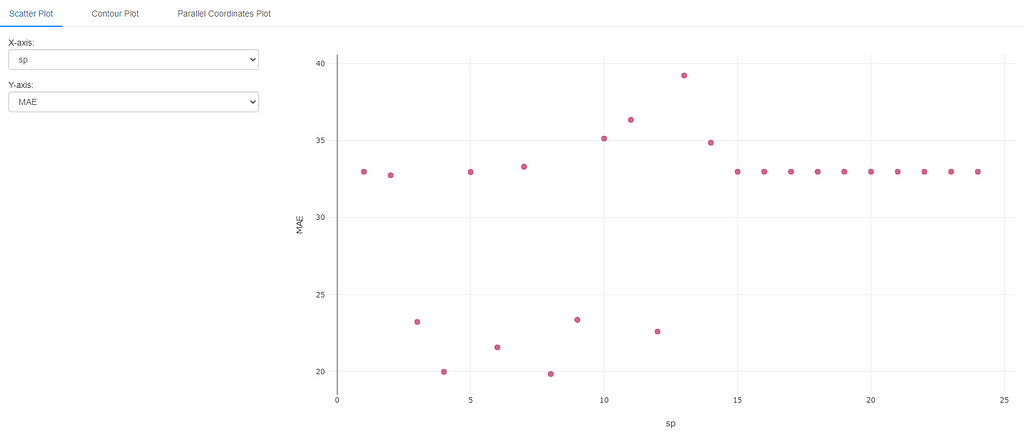
The results of this experiment are a little surprising. While we do get good results at seasonal period =12, we also get good results for seasonal period=3, 4, 6, 8 and 9. This could be due to the fact that for monthly data (like the airline dataset), a period of 3, 6, 9 represent 1, 2, and 3 quarters respectively. These could also be a valid periods over which the data repeats itself. Seasonal period of 4 and 8 are a little harder to explain intuitively, but could represent data repeating itself 3 times a year or 3 times in 2 years respectively (again not completely out of question, though less likely than the other periods).
In any case, this brings about the challenge with hyperparameter intuition and tuning. It is often hard to pin point the “best” hyperparameter ahead of time, but at least we can intuitively set them to a reasonable value. Moreover, as mentioned above, hyperparameters do not tend to work in isolation (univariate). They interact with each other and can affect the model performance in other non-intuitive ways as well. Let’s examine one multivariate case next.
Experimenting with Window Length & Season Period (Multivariate)
In this experiment, we explore the search space taking into consideration window_length and sp simultaneously.
#### Create a model with varying window_length & sp ----
runs = 50
window_lengths = np.random.randint(1, 25, runs)
sps = np.random.randint(1, 25, runs)
for window_length, sp in zip(window_lengths, sps):
    model = exp.create_model(
        "lr_cds_dt", window_length=window_length, sp=sp
    )
MLflow also provides the ability to visualize bi-variate data using a contour plot. In this case, we plot window_length on the x-axis and sp on the y-axis. The color represents the metric of choice (MAE in this case). Lighter shades of blue indicate lower error and hence a better hyperparameter choice in this case.
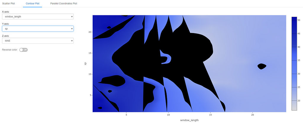
We can see from these results that even in a multivariate setting, anything less than 12 data points for window_length does not give the best results (darker shades of blue). Any values above 12 seem to do reasonably well. For seasonal period, the exact value does not seem to have a very big impact in a bivariate setting as long as window_length is more than 12. (NOTE: in case you are wondering, black areas are the ones where there were not enough sample points to build the contour).
🚀 Conclusion and Next Steps
We can now use this intuition to guide our hyperparameter search space in the future when we encounter similar datasets. Alternately, check out the resources below on how pycaret performs hyperparameter tuning in an optimal and automated manner.
👉 Basic Hyperparameter Tuning for Time Series Models in PyCaret
pycaret also provides the users the option to control the search space during hyperparameter tuning. Users may wish to do this based on manual evaluation as we did in this article. Check out the article below for more details.
👉 Advanced Hyperparameter Tuning for Time Series Models in PyCaret
That’s it for now. If you would like to connect with me (I post about Time Series Analysis frequently), you can find me on the channels below. Until next time, happy forecasting!
📘 GitHub
📗 Resources
- Jupyter Notebook containing the code for this article
Exploring Model Hyperparameter Search Space with PyCaret & MLflow was originally published in Towards Data Science on Medium, where people are continuing the conversation by highlighting and responding to this story.
from Towards Data Science - Medium https://ift.tt/3FIyUWq
via RiYo Analytics


ليست هناك تعليقات