https://ift.tt/3CucCFJ Cleaning and Preparing Marketing Data in R Prior to Modelling or Analysis A basic, step-by-step guide on cleaning t...
Cleaning and Preparing Marketing Data in R Prior to Modelling or Analysis
A basic, step-by-step guide on cleaning typically messy marketing data in R

TLDR
This article looks at a basic workflow for dealing with messy data in R before analysis or inputting into ML models. Specifically it will discuss:
- Importing csv data correctly
- Adding, removing and renaming columns
- Identifying uniques, tackling duplicated values and NAs
- Consistent casing and formatting
- Finding and replacing strings
- Dealing with different date formatting 🙀!
- Merging different datasets into one
- Converting daily data into weekly data
- Turning long data into wide format
I have gone right down to basics, doing this as a step-by-step approach to help new R users get to grips with R, line by line. I hope to turn this into a series on marketing mix modelling in R soon, time permitting 🤗!
The Challenge
For this exercise, I’ve deliberately set the following challenge of:
- Using 2 different data sets, both that can be considered messy
- Sticking with base / default R as much as possible
- Commenting the code as much as possible
Lets get this out of the way first: marketing data is always messy.
Why? Well, it’s because this data is often sat in multiple platforms — some online, some offline, all managed by different teams, external partners and so on. It’s literally all over the place.
Let’s illustrate: if you are an analyst tasked to measure the effectiveness of digital marketing campaigns, you may have to gather data on website performance from Google Analytics, ad performance from Search Ads 360 or Tradedesk, then retrieve customer data and their orders from a CRM or an SQL database.
Accept that there will be incomplete data. There will be NAs or lots of missing values. There will be formatting and structuring problems. Some data might not even be what you think it is (pssst! See that column called “conversions?” That’s not the total enquiries received, it’s actually measuring the number of times users click the “submit enquiry” button — whether or not the enquiry successfully went through is another matter 🙄.)
We’ll need to scrub, clean and whip this data into shape before we can feasibly use it in any modelling or analysis. Let’s do this! 💪
Wrangling with messy data in R
Datasets
For this exercise, we are going to look at two datasets:
- One is daily marketing performance data with typical metrics like date, channel, daily spends, impressions, conversions, clicks etc. We can assume this came from an analytics platform.
- The other is daily sales data (order id, revenue, tax, shipping etc). We can assume this came from a CRM.
- Both datasets can be considered messy (you’ll see why in a minute! 🤭)
👉 You can access the dataset on Kaggle here. Thank you to the dataset owner for kindly letting me use this in the post!
Using base / default R
I’ve decided to deliberately stick with base R as much as I can. Why? Because in using as little R packages as possible, I aim to reduce as much dependencies as I can. When you load an R package, it sometimes also loads additional libraries in the background. There is nothing wrong with this, and part of the beauty of using R is that we can build on the work of others and contribute to the community. However, much of the tasks discussed here can be achieved simply (and sometimes just as quickly), using base R.
Saying that, some functions like View(), str(), aggregate(), merge() are technically not base R. They come from packages that are already loaded by default (e.g. {utils}, {stats}, etc). In this sense, we will consider them default functions and can use them in this challenge.
Also, I honestly think if this is your first try at using R, then learning base R is important before jumping straight onto tidyverse. From experience, I find that having a grounding in R fundamentals super useful.
Commenting as much as possible
I’m going to comment my code as much as possible, line by line, to help make it easier for new R users to learn this. Commenting code should also be good practice btw! Because if you are going to share code templates with your team, it helps them understand what each chunk or line does.
Load the data
We’ve got 2 datasets. Lets download these csvs, load ‘em up in R and see what they look like:
The first line essentially uses the read.csv() function to read the file and then save it to a dataframe called marketing_df.
The View() function in the next line (note the capital “V”) should open up the file in R so you can look at it:
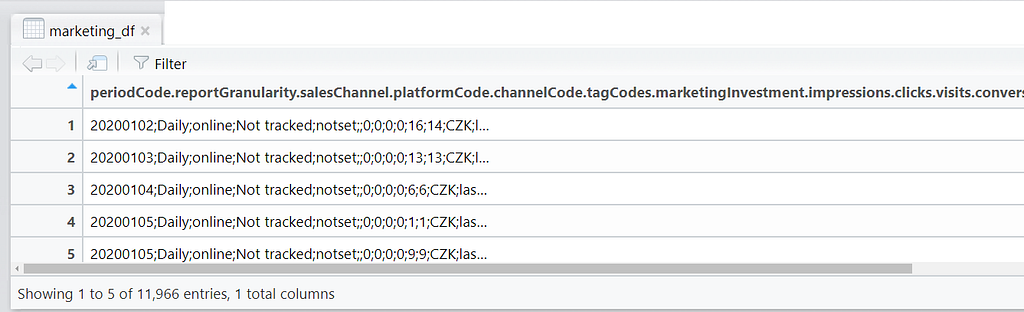
Yuck! The data looks mangled! CSV files can be saved with different separators. By default, CSVs are comma separated (hence the acronym😉) but this one is separated using semicolon as can be seen in the semicolons in the screenshot. Lets load the data again, this time specifying the separator like so:
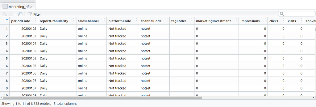
Much better! We can see now each value in their respective columns!
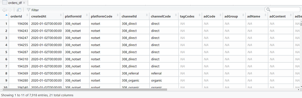
Now that we have dealt with the marketing data, lets get the orders data and save it into a dataframe called orders_df:
Ok great, we’ve loaded both datasets. Clearly we can see there is work to be done to clean ‘em up. Let’s tackle the marketing dataset first and then we’ll work on the orders dataset.
Cleaning the marketing data
The marketing_df dataframe has many useful columns. For illustration purposes, let’s say we only care about the following 3 columns:
- periodCode (1st column)
- platformCode (4th column)
- marketingInvestment (7th column).
We will grab these columns and save them to a new dataframe called marketing_df_clean. We also want to rename the columns with names that are easier to understand.
Let’s go:
So we’ve turned the dataframe from this:
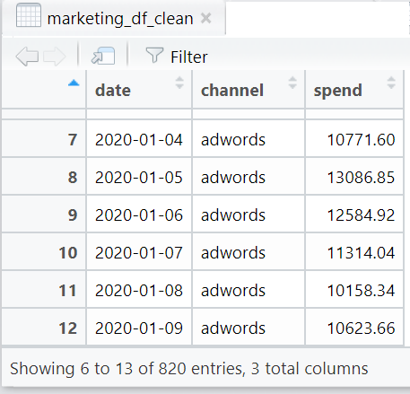
to this 👇
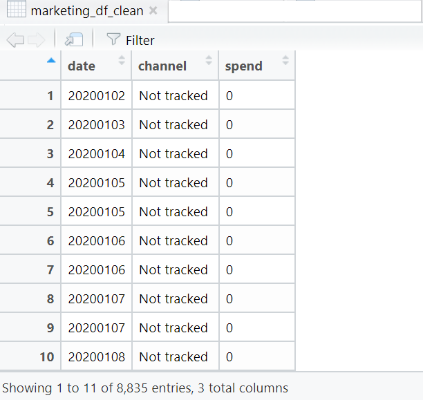
We’ve saved this into a smaller dataframe called marketing_df_clean with only 3 columns. Have look at the data, scroll and pay attention to how the values are presented. There’s a couple of things you’ll notice:
- The dates are weird. I mean, we recognise them as dates of course, but they could be read by R as anything but. We need to standardise them into a proper date format.
- The values in the channel column have got all sorts of casing. Let’s force them all to lowercased to keep them consistent.
Also some of the values need updating and this is where domain knowledge comes in handy: since paid media is already defined (e.g. Facebook, Adwords) then “unpaid” can be taken as “organic”. “Not tracked” can mean “direct”, and “silverpop” is an email platform so can be renamed to “email”. - And if you review the Spend column closely, you’ll also notice that values are comma separated. E.g. 20,29.
You can check how R reads these values by running this line:
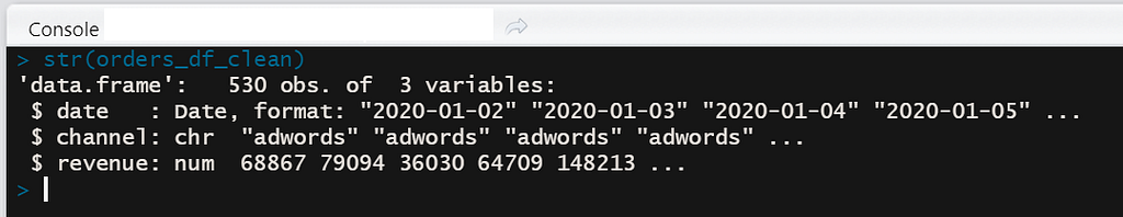
str(marketing_df_clean)
This str() function shows you how R sees the internal structure of an R object, in this case a dataframe of 3 columns:
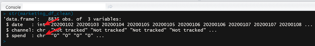
This output shows that R wrongly read the date column as an integer instead of format date. Spend is read as character which is incorrect! Spend should be numeric. It is likely because of the commas between digits that is causing this to be read as text.
Based on the above, we know we need to do the following:
- Format the date column so that it is recognised as dates properly. Unfortunately, date formatting is a real pain 😡. And so for this part, I will be using the fantastic {lubridate} package to coerce these dates into the right format. I think it’s the only non-base / non-default package I am using in this exercise to be fair. We’ll sort dates out last.
- Force lowercase all text values in the Channel column
- Once lowercased, inspect the Channel column, look at all the possible unique values available
- Pick out the channels we want to rename
- Finally, make sure the column for Spend is recognised as numeric.
Here goes:
And then, in the wise words of StatQuest’s Josh Starmer:
Bam!!! 💥
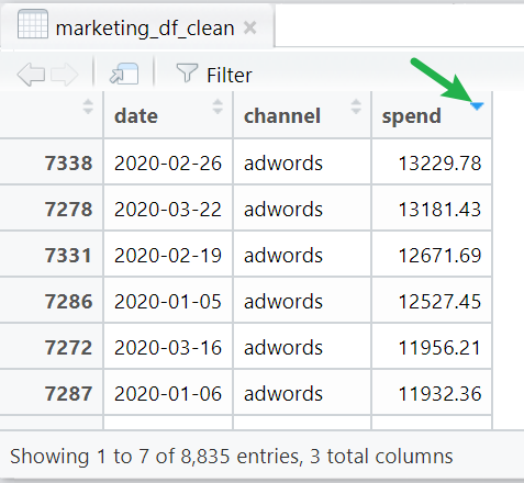
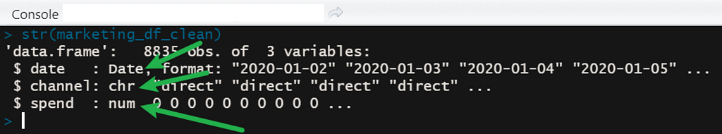
Dates are now formatted correctly and recognised as such. Spend is now correctly identified as numeric. We’re in business!!
Erm, actually not quite. Look at the data again - it seems there are duplicate rows (e.g. same channel, same day).
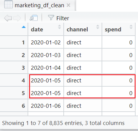
We want make sure there is only 1 channel per day, and the spend is the total spend for that channel in that day. Recall that we’ve dropped other columns we don’t need earlier on. Those columns were there to segment the data further (e.g. by desktop or mobile). When we drop those columns we need to remember to sum the Spend by channel for that given day.
The aggregate() function does this very well:
marketing_df_clean <- aggregate(spend ~ date + channel, data = marketing_df_clean, sum)
Which now gives us a nice table like this:
Yay! We’ve now got a clean data set of spends per channel each day.
Cleaning the orders data
Now lets do the same steps we have done above, but this time with the orders data. To remind ourselves, the orders_df dataframe looks like this:
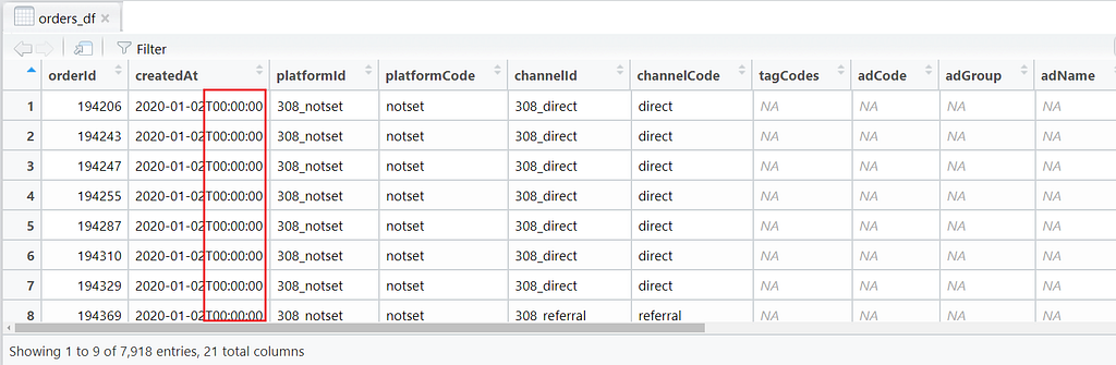
For this exercise, we only care about the createdAt (2nd), platformCode (4th) and revenue (18th) columns.
Notice also that the date has these timestamps appended to them. We’ll need to strip these out first before we can use {lubridate} to format the date to the consistent year-month-day format we’ve used earlier.
Apart from that, we can use the same workflow we’ve done for the marketing data onto this orders data, like so:
Which should result in this clean table:
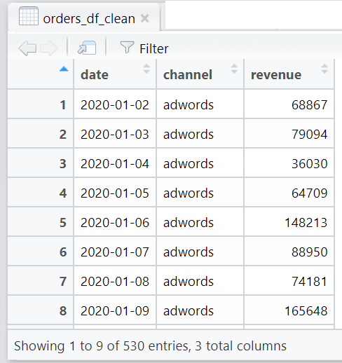
R is also recognising the date column as date format and revenue is numeric. The orders data is now done! With both marketing and orders data sorted, we can now move on to converting them into a weekly dataset.
Converting daily data into weekly data
There are many reasons why you might want to convert a daily dataset into a weekly one. In marketing mix modelling and general forecasting for digital marketing, it is common to use weekly data because not all channels can have an immediate impact on sales on the same day, conversions might occur on the 2nd, 3rd or 4th day after initial impression.
We can do this very easily in R.
- First, we’ll create a new column called “week”. This will represent the week of the year in which the date falls on. E.g. 2020–03–15 falls on Week 11 of the year 2020. (I find this site really helpful to check weeks quickly.)
- Then we’ll create a new column called “monthyear”. For the date 2020–03–15, month year will output “03–2020”.
- We’ll do this for both the marketing and orders data 👇
You should now have 2 new dataframes.
marketing_df_weekly:
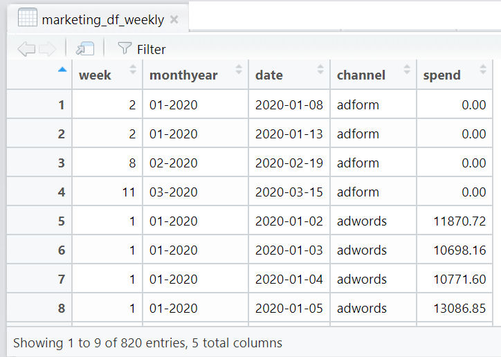
And orders_df_weekly:
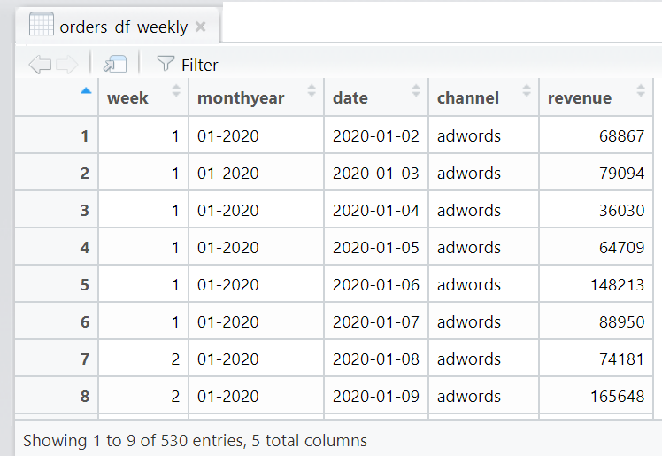
As you can see, the values are not yet aggregated and summed by week. We simply introduced 2 new columns in each dataframe to tell us what week each specific date falls under.
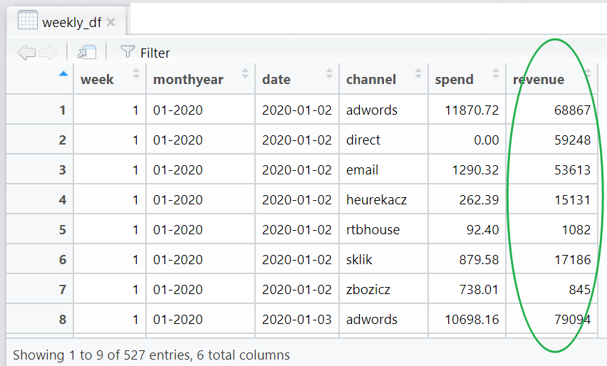
Next, we’ll join the marketing and the orders data into one dataframe we’ll call weekly_df. We do this using the merge() function:
weekly_df <- merge(marketing_df_weekly, orders_df_weekly)
View(weekly_df)
Using the above line should give us this 👇 — a table with spend, and now also revenue, by channel, for each day. The columns “week” and “monthyear” gives you an indication of the week number and month the date falls under.
Now, we can aggregate spends and revenue by week like so:
- Sum all spends per week by channel. Save it into a dataframe called weekly_spend_df
- Sum all revenue per week by channel. Save it into a dataframe called weekly_rev_df
- Get the first date of each week, call this column “weekdatestart” and save into a dataframe called weekly_df_dates. Removing any duplicate rows.
- Merge these 3 dataframes together into a clean, weekly aggregated dataframe called weekly_df_updated.
Fab! You should now get a dataframe that looks like this:
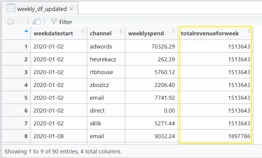
Hang on! Do you notice anything odd with this 🤔?
The totalrevenuefortheweek is, as the name says, the total revenue for that week as defined in the following line:
weekly_rev_df <- aggregate(revenue ~ week, data = weekly_df, sum)
However, weeklyspend refers to the total spend for the specific channel for the given week, defined here:
weekly_spend_df <- aggregate(spend ~ week + channel, data = weekly_df, sum)
Looking at the above table, it makes it seem like spending £70,326.29 on “adwords” on week beginning 2nd Jan 2020 yielded £1,513,643 in revenue. For the same week period, spending £262.32 on the “heurekacz” channel yielded another £1,513,643 in revenue! And so on.
👎 This is of course, incorrect!
What we mean to show is that the combined performance of spending on adwords, email, rtbhouse and the other channels for that given week, have all together, yielded a revenue of £1,513,643 for that week.
To see this properly, we need to turn this long data format into wide data format.
Converting long data into wide data
Turning long data into wide data and vice versa is pretty straightforward! The base reshape() function lets you do just that in one line of code, like so:
weekly_reshaped_channel <- reshape(weekly_df_updated, idvar = c("weekdatestart","totalrevenueforweek"), timevar = "channel", direction = "wide")
When you View(weekly_reshaped_channel), you should see the following table:
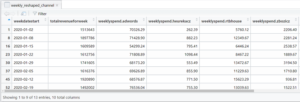
This makes better sense as you can see total revenue achieved for each week and the spends by each channel for that week!
Dealing with NAs
You can use print() to view the data in console and check for NA values. Or simply use View() if you prefer to look at it spreadsheet-style as we have done in this exercise:
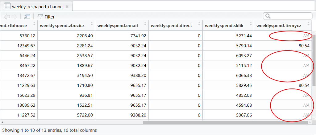
If NAs are detected, you can replace NA values with 0 using is.na(), like so:
#view the data and check for NA or missing values
print(weekly_reshaped_channel)
#if found, replace any NA with 0
weekly_reshaped_channel[is.na(weekly_reshaped_channel)] <- 0
#check
str(weekly_reshaped_channel)
View(weekly_reshaped_channel)
The end
👏Well done on getting right to the end! We’ve FINALLY got the dataset we need which we can use to perform modelling later.
The full R code
👉 Get the full R code from my Github repo here.
I hope you have found this post useful in some way. No doubt there are much quicker and better ways to achieve the same end results but the intention of this post is to get right down to basics and help new R users get to grips with R. If you have done a similar exercise and found a better way, please do share in the comments 🤗!
I am also thinking of continuing the next post using this same data for marketing mix modelling. We shall see. TTFN!
Cleaning and preparing marketing data in R prior to machine learning or analysis was originally published in Towards Data Science on Medium, where people are continuing the conversation by highlighting and responding to this story.
from Towards Data Science - Medium https://ift.tt/3x3cewM
via RiYo Analytics


No comments