https://ift.tt/3nlHtQE Comparing ThymeBoost, Pmdarima, and Prophet Image by Pietro Mattia on Unsplash TLDR: When comparing ThymeBoos...
Comparing ThymeBoost, Pmdarima, and Prophet

TLDR: When comparing ThymeBoost to a few other popular time-series methods, we find that it can generate very competitive forecasts. Spoiler warning: ThymeBoost wins. But beyond winning, we see that there are many benefits of the ThymeBoost framework, even in the cases where it loses.
For more examples you can view the ThymeBoost Github.
First post in the series: Time Series Forecasting with ThymeBoost. If you haven’t viewed it yet then check it out!
Introduction
The examples used in this competition are fairly popular, but some of the code used for data wrangling has been taken from this article (thanks Tomonori Masui!). You should check out the article to see how a few other models perform on these datasets.
The first example is a fairly well known time-series: the Airline Passenger dataset. This data is widely available and one source is from Kaggle or from the Github. Make sure you have the latest ThymeBoost package which can be installed via pip:
pip install ThymeBoost --upgrade
Now that we are up-to-date, let’s take a look!
Airline Passenger Dataset
import numpy as np
import pandas as pd
from matplotlib import pyplot as plt
from ThymeBoost import ThymeBoost as tb
import seaborn as sns
sns.set_style("darkgrid")
#Airlines Data, if your csv is in a different filepath adjust this
df = pd.read_csv('AirPassengers.csv')
df.index = pd.to_datetime(df['Month'])
y = df['#Passengers']
plt.plot(y)
plt.show()
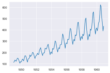
This time series is quite interesting! A clear trend along with multiplicative seasonality. Definitely a good benchmark for any forecasting methodology.
In order to judge the forecasting methods, we will split the data into a standard train/test split where the last 30% of the data is held out. The outcome of the testing procedure can change depending on this split. In an attempt to remain unbiased, the train/test splits from the aforementioned article will be used.
Any tuning or model selection will be done on the training set while the test set will be used to judge the methods. The goal (at least for me) is to see if ThymeBoost can be competitive against other vetted methods. If you were to implement a forecasting model in production, then you may want to use a more robust method to judge models such as time-series cross validation.
test_len = int(len(y) * 0.3)
al_train, al_test = y.iloc[:-test_len], y.iloc[-test_len:]
First, let’s try out an Auto-Arima implementation: Pmdarima.
import pmdarima as pm
# Fit a simple auto_arima model
arima = pm.auto_arima(al_train,
                      seasonal=True,
                      m=12,
                      trace=True,
                      error_action='warn',
                      n_fits=50)
pmd_predictions = arima.predict(n_periods=len(al_test))
arima_mae = np.mean(np.abs(al_test - pmd_predictions))
arima_rmse = (np.mean((al_test - pmd_predictions)**2))**.5
arima_mape = np.sum(np.abs(pmd_predictions - al_test)) / (np.sum((np.abs(al_test))))
Next, we will give Prophet a shot.
from fbprophet import Prophet
prophet_train_df = al_train.reset_index()
prophet_train_df.columns = ['ds', 'y']
prophet = Prophet(seasonality_mode='multiplicative')
prophet.fit(prophet_train_df)
future_df = prophet.make_future_dataframe(periods=len(al_test), freq='M')
prophet_forecast = prophet.predict(future_df)
prophet_predictions = prophet_forecast['yhat'].iloc[-len(al_test):]
prophet_mae = np.mean(np.abs(al_test - prophet_predictions.values))
prophet_rmse = (np.mean((al_test - prophet_predictions.values)**2))**.5
prophet_mape = np.sum(np.abs(prophet_predictions.values - al_test)) / (np.sum((np.abs(al_test))))
Finally, implementing ThymeBoost. Here we are using a new method: ‘autofit’ from the latest version of the package. This method will try several simple implementations given a possible seasonality. It is an experimental feature and only works for traditional time-series. A current issue is that it tries several redundant parameter settings, this will be fixed in a future release, speeding up the process! Additionally, if you intend to pass exogenous factors we recommend using the optimize method found in the README instead.
boosted_model = tb.ThymeBoost(verbose=0)
output = boosted_model.autofit(al_train,
                               seasonal_period=12)
predicted_output = boosted_model.predict(output, len(al_test))
tb_mae = np.mean(np.abs(al_test - predicted_output['predictions']))
tb_rmse = (np.mean((al_test - predicted_output['predictions'])**2))**.5
tb_mape = np.sum(np.abs(predicted_output['predictions'] - al_test)) / (np.sum((np.abs(al_test))))
By setting verbose=0 when building the class it silences the logging of each individual model. Instead, a progress bar will be displayed to denote progress through the different parameter settings as well as the ‘optimal’ settings found. By default, ThymeBoost’s autofit method will do 3 rounds of fitting and forecasting. This process rolls through the last 6 values of the training set to choose the ‘best’ settings. For this data, the optimal settings found were:
Optimal model configuration: {'trend_estimator': 'linear', 'fit_type': 'local', 'seasonal_period': [12, 0], 'seasonal_estimator': 'fourier', 'connectivity_constraint': True, 'global_cost': 'maicc', 'additive': False, 'seasonality_weights': array([1., 1., 1., 1., 1., 1., 1., 1., 1., 1., 1., 1., 1., 1., 1., 1., 1.,
       1., 1., 1., 1., 1., 1., 1., 1., 1., 1., 1., 1., 1., 1., 1., 1., 1.,
       1., 1., 1., 1., 1., 1., 1., 1., 1., 1., 1., 1., 1., 1., 1., 1., 1.,
       1., 1., 1., 1., 1., 1., 1., 1., 1., 1., 1., 1., 1., 1., 1., 1., 1.,
       1., 1., 1., 1., 1., 1., 1., 1., 1., 5., 5., 5., 5., 5., 5., 5., 5.,
       5., 5., 5., 5., 5., 5., 5., 5., 5., 5., 5., 5., 5., 5., 5., 5.]), 'exogenous': None}
Params ensembled: False
Some important things to note:
- ‘additive’ is set to false, meaning that the entire process is ‘multiplicative’ i.e. the log is taken of the input series. Normal ‘multiplicative’ seasonality is not yet implemented.
- There is an array of ‘seasonality_weights’ where the last 2 ‘seasonal_periods’ are set to 5, meaning those periods impact the seasonality component 5 times more than the other periods.
- ‘seasonal_period’ is [12, 0] so it cycles back and forth between measuring seasonality and not measuring it. This is interesting behavior but it essentially adds some regularization to the seasonality component.
Speaking of components, let’s take a look:
boosted_model.plot_components(output, predicted_output)
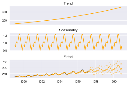
All in all, ThymeBoost decided to take the log of the input series, fit a linear changepoint model, and add a ‘changepoint’ to the seasonality component.
Were these correct decisions? Let’s take a look at the error metrics:
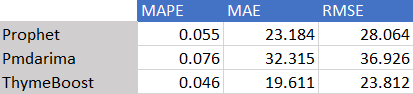
These error metrics speak for themselves, ThymeBoost outperformed the other methods across the board. But what do the forecasts actually look like?
plt.plot(pmd_predictions, label='Pmdarima')
plt.plot(al_test.values, label='Actuals')
plt.plot(prophet_predictions.values, label='Prophet')
plt.plot(predicted_output['predictions'].values, label='ThymeBoost')
plt.legend()
plt.show()
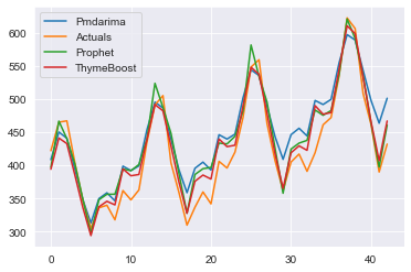
Clearly, all methods picked up very similar signals. It seems as though ThymeBoost was just slightly better in terms of the seasonal shape, potentially due to the seasonal weighting it decided to use.
WPI Dataset
The next dataset is the U.S. Wholesale Price Index (WPI) from 1960 to 1990 and once again the example is taken from the aforementioned article.
This dataset unfortunately does not come with ThymeBoost but we can access it via Statsmodels:
from statsmodels.datasets import webuse
dta = webuse('wpi1')
ts_wpi = dta['wpi']
ts_wpi.index = pd.to_datetime(dta['t'])
test_len = int(len(ts_wpi) * 0.25)
ts_wpi = ts_wpi.astype(float)
wpi_train, wpi_test = ts_wpi.iloc[:-test_len], ts_wpi.iloc[-test_len:]
plt.plot(ts_wpi)
plt.show()
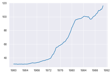
This time-series is fairly different than the previous. It appears to lack any seasonality so those settings will be disabled (although if we accidentally feed seasonality settings to ThymeBoost it does not change much).
Let’s follow the same process as before and first fit Pmdarima:
import pmdarima as pm
# Fit a simple auto_arima model
arima = pm.auto_arima(wpi_train,
                      seasonal=False,
                      trace=True,
                      error_action='warn',
                      n_fits=50)
pmd_predictions = arima.predict(n_periods=len(wpi_test))
arima_mae = np.mean(np.abs(wpi_test - pmd_predictions))
arima_rmse = (np.mean((wpi_test - pmd_predictions)**2))**.5
arima_mape = np.sum(np.abs(pmd_predictions - wpi_test)) / (np.sum((np.abs(wpi_test))))
Next, Prophet:
from fbprophet import Prophet
prophet_train_df = wpi_train.reset_index()
prophet_train_df.columns = ['ds', 'y']
prophet = Prophet(yearly_seasonality=False)
prophet.fit(prophet_train_df)
future_df = prophet.make_future_dataframe(periods=len(wpi_test))
prophet_forecast = prophet.predict(future_df)
prophet_predictions = prophet_forecast['yhat'].iloc[-len(wpi_test):]
prophet_mae = np.mean(np.abs(wpi_test - prophet_predictions.values))
prophet_rmse = (np.mean((wpi_test - prophet_predictions.values)**2))**.5
prophet_mape = np.sum(np.abs(prophet_predictions.values - wpi_test)) / (np.sum((np.abs(wpi_test))))
And finally, ThymeBoost:
boosted_model = tb.ThymeBoost(verbose=0)
output = boosted_model.autofit(wpi_train,
                               seasonal_period=0)
predicted_output = boosted_model.predict(output, forecast_horizon=len(wpi_test))
tb_mae = np.mean(np.abs((wpi_test.values) - predicted_output['predictions']))
tb_rmse = (np.mean((wpi_test.values - predicted_output['predictions'].values)**2))**.5
tb_mape = np.sum(np.abs(predicted_output['predictions'].values - wpi_test.values)) / (np.sum((np.abs(wpi_test.values))))
And the optimal settings, which also can be accessed directly through:
print(boosted_model.optimized_params)
which returns:
{'trend_estimator': 'linear', 'fit_type': 'local', 'seasonal_period': 0, 'seasonal_estimator': 'fourier', 'connectivity_constraint': False, 'global_cost': 'mse', 'additive': True, 'exogenous': None}
Like last time, ThymeBoost chose a linear model with local fit a.k.a. a linear changepoint model for the trend component. Except this time ‘connectivity_constraint’ is set to False which relaxes that the trend lines at the changepoint connect AT the changepoint.
Let’s take a look at the error metrics:
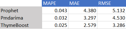
Once again ThymeBoost outperforms the other two methods.
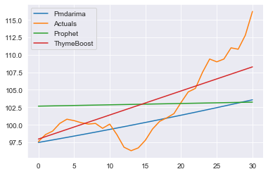
And the forecasts:
plt.plot(pmd_predictions, label='Pmdarima')
plt.plot(wpi_test.values, label='Actuals')
plt.plot(prophet_predictions.values, label='Prophet')
plt.plot(predicted_output['predictions'].values, label='ThymeBoost')
plt.legend()
plt.show()
Conclusion
The goal of this article was to see if ThymeBoost can compete against other popular methods, it clearly can in these instances. But don’t be fooled into thinking ThymeBoost is a panacea (although I wish it was!). There are many times where it is outperformed, however, one major benefit is that any method which outperforms ThymeBoost could potentially be added into the framework. Once a method is added, it gains access to some interesting features via the boosting process.
An example of this can be found in the article already referenced. For the sunspots dataset, ThymeBoost’s autofit does not do any ARIMA modelling so it has poor results compared to the ARIMA(8, 0, 1) found from sktime. However, if we use the standard fit method and pass that ARIMA order with a local fit (so we allow changepoints) we outperform sktime’s Auto-ARIMA.
I will leave that as an exercise for you to try, simply use these settings:
output = boosted_model.fit(sun_train.values,
                           trend_estimator='arima',
                           arima_order=(8, 0, 1),
                           global_cost='maicc',
                           seasonal_period=0,
                           fit_type='local'
                           )
As mentioned before, this package is still in early development. The sheer number of possible configurations makes debugging an involved procedure, so use at your own risk. But please, play around and open any issues you encounter on GitHub!
Auto-Forecasting in Python with ThymeBoost was originally published in Towards Data Science on Medium, where people are continuing the conversation by highlighting and responding to this story.
from Towards Data Science - Medium https://ift.tt/30ATdWT
via RiYo Analytics


ليست هناك تعليقات