https://ift.tt/3nUB27q Model Interpretability How to design an interpretable machine learning process Image of kiquebg from Pixabay . ...
Model Interpretability
How to design an interpretable machine learning process

I know this topic has been discussed many times. But I recently gave some talks on interpretability (for SCAI and France Innovation) and thought it would be good to include some of my work in this article. The importance of explainability for the decision-making process in machine learning doesn’t need to be proved any longer. Users are demanding more explanations, and although there are no uniform and strict definitions of interpretability and explainability, the number of scientific papers explaining artificial intelligence (or XAI) is growing exponentially.
As you may know, there are two ways to design an interpretable machine learning process. Either you design an intrinsically interpretable predictive model, for example with rule-based algorithms, or you use a black-box model and add a surrogate model to explain it. The second way is called post-hoc interpretability. There are two types of post-hoc interpretable models: global models to describe the average behaviour of your black-box models, or local models to explain individual predictions. Nowadays, there are several tools for creating a post-hoc interpretable model, most of them are model-agnostic, i.e. they can be used independently of the algorithm used.
I will present the most common of them. This article in based on the reference book of Christoph Molnar: Interpretable Machine Learning. To illustrate the methods, I use the usual Boston Housing dataset. The target is the median price of owner-occupied homes in $1000's.
Partial Dependence Plot (PDP).
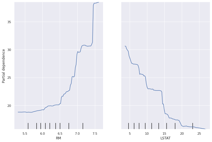
PDP is a global, model-agnostic interpretation method. This method shows the contribution of individual features to the predictive value of your black box model. It can be applied to numerical and categorical variables. First, we choose a feature and its grid values (the range of the chosen feature). Then the values of this feature are replaced by grid values and the predictions are averaged. For each value of the grid, there is a point corresponding to an average of the predictions. Finally, the curve is drawn. The main limitation is that humans are not able to understand a graph with more than three dimensions. Therefore, we cannot analyse more than two features in a partial dependency diagram.

feature RM and LSTAT. Image from the author.
In these graphs, we can see the average impact of the average number of rooms per dwelling (RM) and the percentage of the lower class in the population (LSTAT) on the median price. For example, we can deduce that the lower the number of rooms, the lower the median price (this seems coherent).
The function plot_partial_dependence is already implemented in the inspection module of the package scikit-learn.
Accumulated Local Effects (ALE).
ALE is also a global, model-agnostic interpretation method. It is an alternative to PDP, which is subject to bias when variables are highly correlated. For example, the variable RM, which indicates the number of rooms, is highly correlated with the area of the house. So RM=7.5 would be an unrealistic individual for a very small area. The idea behind ALE is to consider instances with a similar value of the chosen variable, rather than substituting values for all instances. When you average the predictions, you get an M-plot. Unfortunately, the M-plots represent the combined effect of all correlated characteristics. To get a better understanding, I quote the example from Interpretable Machine Learning:
“Suppose that the living area has no effect on the predicted value of a house, only the number of rooms has. The M-Plot would still show that the size of the living area increases the predicted value, since the number of rooms increases with the living area.”
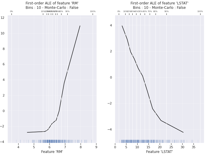
ALE computes the differences of the predictions instead of the average regarding a small window (e.g. using empirical quantiles). In the following example, I plot the ALE for the features RM and LSTAT with 10 windows.

feature RM and LSTAT. Image from the author.
The vertical lines represent the windows under consideration. The empirical quantiles are designed so that 10 % of the individuals lie in each window. Unfortunately, there is no solution to set the number of bins, which strongly influences the interpretation.
For the illustration, I have used the open-source package ALEPython available on Github.
Individual Conditional Expectation (ICE).
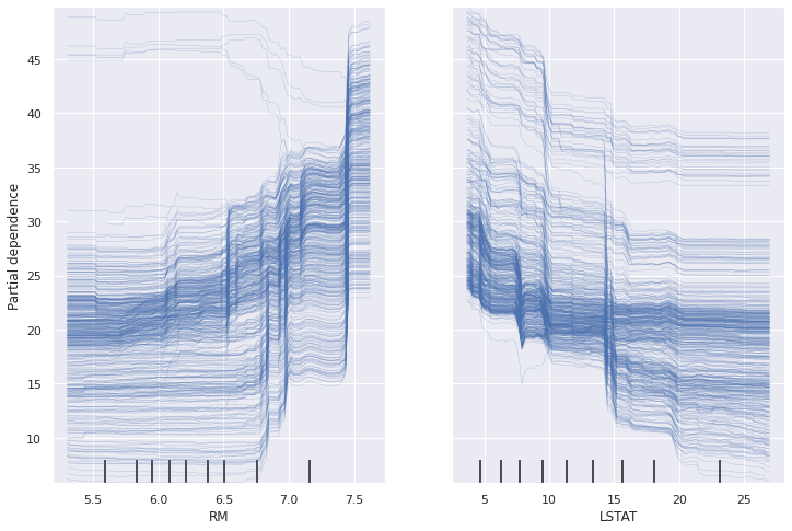
ICE is a local, model-agnostic interpretation method. The idea is the same as the PDP but instead of plotting the average contribution, we plot the contribution for each individual. Of course, the main limitation is the same as PDP. Moreover, if you have too many individuals, the plot may become unexplainable.

feature RM and LSTAT. Image from the author.
Here we see the effects of the average number of rooms per dwelling (RM) and the percentage of lower class in the population (LSTAT) on the median price for each of the 506 observations. Again, we can see that the lower the number of rooms, the lower the median price. However, there are 5 individuals for whom RM shows an opposite behaviour. These 5 individuals should be carefully examined as they could indicate an error in the database.
The function plot_partial_dependence is already implemented in the inspection module of the package scikit-learn.
Local Interpretable Model-agnostic Explanations (LIME).
LIME, as its name suggests, is a local model-agnostic interpretation method. The idea is simple, from a new observation LIME generates a new dataset consisting of perturbed samples and the corresponding predictions of the underlying model. Then, an interpretable model is fitted on this new dataset, which is weighted by the proximity of the sampled observation to the observation of interest.

chosen observation is the 42nd and the surrogate local model is a RIDGE regression. Image from the author.
In this visual output of LIME, the prediction for the 42nd observation is explained. In the created data set, the predicted values range from 8.72 to 47.73. The predicted value for the interset observation is 24.99. We can see that the value of LSTAT has a positive influence on the prediction, which confirms the previous conclusions from PDP and ICE.
SHapley Additive exPlanations (SHAP).
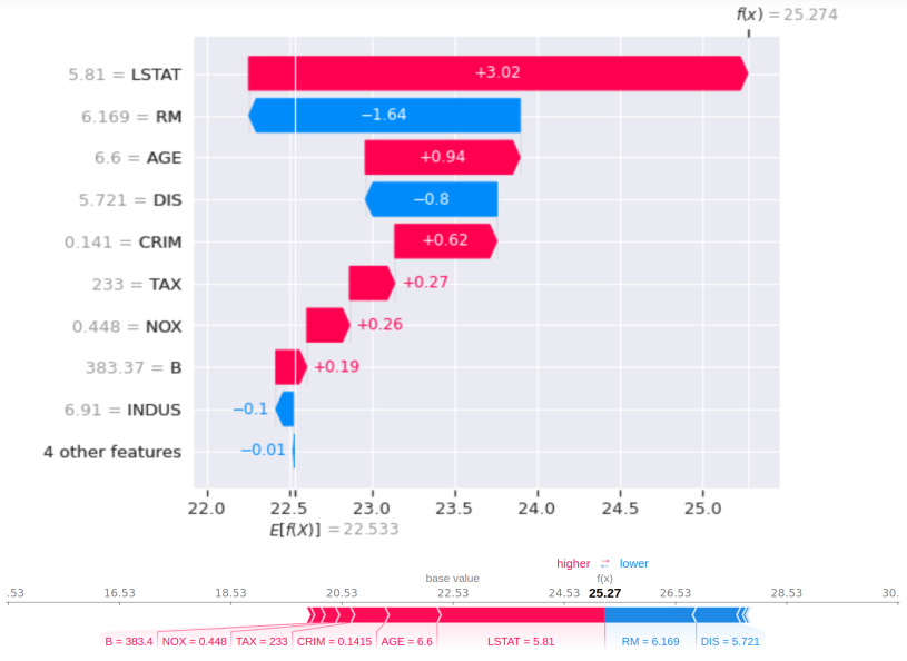
SHAP is a local model-agnostic interpretation method based on the Shapley value. The Shapley value comes from game theory, and there are several articles on Toward Data Science and others that talk about it. I just want to remind you here that in this context, the game is collaborative, and the task is prediction, the gain is the distance between the prediction and a baseline prediction (usually the average of observations), and the players are the features. Then, the Shapley value is used to separate the prediction shift from the baseline prediction among the features. So, each feature’s realization implies a variation of the prediction, positively or negatively. The idea behind SHAP is to represent the Shapley value explanation as an additive feature attribution method. Hence, it becomes a linear model, where the intercept is the baseline prediction. The following graphical representation of SHAP applied to a XGBoost illustrates these explanations.

chosen observation is the 42nd. Image from the author.
In this figure, we see the influence of each variable on the 42nd prediction. Here, the baseline prediction is 22.533. Then the variable INDUS=6.91 shifts the prediction by -0.1, the variable B=383.37 shifts the prediction by +0.19, and so on. We see that the largest shifts come from the variables LSTAT and RM, which are the most important features of this dataset.
Conclusion
Local models are used more often than the global models. If you want a global description of your model, it is best to use a predictive algorithm that is interpretable in itself. These are not the most accurate algorithms, but they do allow for an overall description of the generated model. If you want a very accurate predictive model, you usually want to be able to explain each prediction individually rather than just the overall model. For example, an algorithm for a self-driving car should be able to explain each of its predictions in case of an accident.
In order to be concise, I have omitted to present the feature importance, the feature interaction, the second-order ALE, the KernelSHAP and others methods. I have only taken a brief overview to show you what is available today to interpret your black box models. If you want to learn more about this topic, I recommend the book of Christoph Molnar: Interpretable Machine Learning.
About Us
Advestis is a Contract Research Organization (CRO) with a deep understanding and practice of Interpretable AI and Machine Learning techniques.
LinkedIn: https://www.linkedin.com/company/advestis/
A Brief Overview of Methods to Explain AI (XAI) was originally published in Towards Data Science on Medium, where people are continuing the conversation by highlighting and responding to this story.
from Towards Data Science - Medium https://ift.tt/3xt8Lb2
via RiYo Analytics

No comments