https://ift.tt/3G46d7f Everybody knows what Gradient Descent is and how it works. Ever wondered why it works? Here’s a mathematical explana...
Everybody knows what Gradient Descent is and how it works. Ever wondered why it works? Here’s a mathematical explanation

What is Gradient Descent?
Gradient descent is an iterative optimization algorithm that is used to optimize the weights of a machine learning model (linear regression, neural networks, etc.) by minimizing the cost function of that model.
The intuition behind gradient descent is this: Picture the cost function (denoted by f(Θ̅ ) where Θ̅ =[Θ₁, … Θₙ]) plotted in n dimensions as a bowl. Imagine a randomly placed point on that bowl represented by n coordinates (this is the initial value of your cost function). The minimum of this “function” then will be the bottom of the bowl.
The goal is then to reach to the bottom of the bowl (or minimize the cost) by progressively moving downwards on the bowl. For this to happen, we should know the slope of the bowl in different directions from where the point currently is, so that we can decide which direction to move in for fastest convergence. To determine this, we calculate the gradient of the function at that point. On iteratively doing this, we will eventually reach some minimum-valued point and the coordinates of that point will be the optimal weights of the model.
How Gradient Descent Works
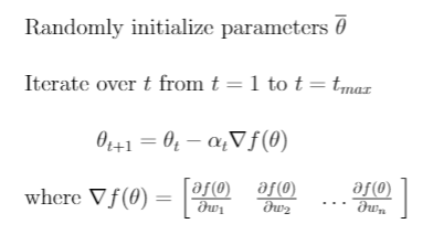
Here is a more formal definition of Gradient Descent:
Starting with the input matrix X which represents the list of n-dimensional input vectors and an initial value to the weights Θ̅, we know that in the linear regression equation is given by: y̅ = Θ̅ᵗX. Now, if the cost function is given by f(Θ̅ ), this is how we formulate Gradient Descent:

Here, t is the iteration counter and tₘₐₓ is the maximum number of iterations we run the loop for.
Why it Works
The first question here should be: The second derivative test and hence the second derivative of any function f(Θ̅) when equated to zero tells you whether Θ̅ is a local maximum or a local minimum of that function. Now, since we are interested in minimizing, we can reverse engineer this concept and solve for Θ̅ given the second derivative of f(Θ̅) is negative.
So, why do we not do that and instead solve the minimization problem iteratively (as in gradient descent)? Well, the answer lies in the fact that first and foremost, the second derivative is not guaranteed to always exist. Second, the computational complexity of solving the second derivative equation for Θ̅ₘᵢₙ is very high. In fact, sometimes it is not possible to solve using calculus, and has to be solved numerically.
The Minimization Problem
So, specifying the general minimization problem numerically (and hence iteratively), we say that Θ̅ₜ₊₁ = Θ̅ₜ + dₜ where dₜ is some general direction of minimization (look back at the bowl example) at time t

Now, to choose the appropriate dₜ so that Θ̅ₜ₊₁ < Θ̅ₜ — and we move towards minimization.
Taylor Series
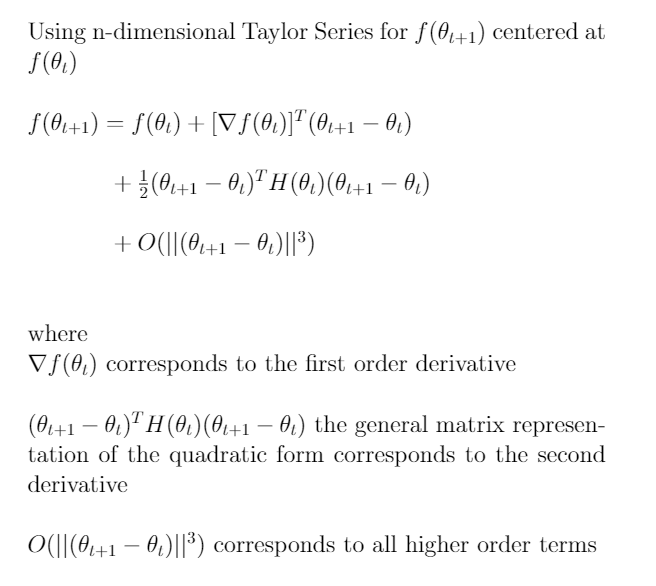
To solve the above minimization problem, we make use of the Taylor series for n dimensions. We calculate the f(Θ̅ₜ₊₁) using the Taylor series centered at f(Θ̅ₜ). This is what it looks like:


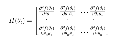
Here the matrix H is the Hessian matrix, representing the second-order partial derivative of the function f(Θ̅ₜ)
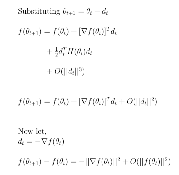
Next, we substitute the equation from the definition of minimization: Θ̅ₜ₊₁ = Θ̅ₜ + dₜ

In the above image, we incorporate the cubic terms in the asymptotic term itself since we only want to work with the first two terms and we get O(||dₜ||²). Next, as mentioned before we try to choose the direction of minimization dₜ that will give us f(Θ̅ₜ₊₁) < f(Θ̅ₜ) and hence lead us towards minimization over t time steps.
We select dₜ to be the negative of the gradient of the cost function at time t — and the similarity to gradient descent starts to appear, and we obtain the last line. Now, notice that in the equation on the last line above, the first and the second term are similar to each other and the end result of that can either be positive or negative. This actually depends on the higher order terms encapsulated within the asymptotic bound. To make sure that we end up with a negative value on the right and a decreasing value over time, we introduce a new term α.
…and Viola!

You guessed it right! α is the learning rate that we normally see in Gradient Descent. Introducing α and making sure that it is very less guarantees that the second term in the final equation above is always less than the first term and hence, we get a negative result on the right hand side. This, in turn ensures that we minimize the function f(Θ̅) over time t
This article is inspired by the lecture series of Dr. Cowan at Rutgers University.
You can find the Latex file for the equations here. I’d love to connect on Linkedin!
Why Gradient Descent Works? was originally published in Towards Data Science on Medium, where people are continuing the conversation by highlighting and responding to this story.
from Towards Data Science - Medium https://ift.tt/3aTrJgI
via RiYo Analytics

No comments