https://ift.tt/2ZejCJp Clustering its benefits. Clustering time series data before fitting can improve accuracy by ~33% — src . Figure ...
Clustering its benefits.
Clustering time series data before fitting can improve accuracy by ~33% — src.
In 2021, researchers at UCLA developed a method that can improve model fit on many different time series’. By aggregating similarly structured data and fitting a model to each group, our models can specialize.
While fairly straightforward to implement, as with any other complex deep learning method, we are often computationally limited by large data sets. However, all of the methods listed have support in both R and python, so development on smaller datasets should be pretty “simple.”
In this post we’ll start with a technical overview then get into the nitty gritty of why clustering improves the fit of time series forecasts. Let’s dive in…
1 — Technical TLDR
Effective preprocessing and clustering can improve neural network forecasting accuracy on sequential data. The paper contributes to each of the following areas:
- Removing outliers by leveraging LOESS and the tsclean package in R.
- Imputing missing data using k-nearest neighbors.
- Clustering using both distance and feature-based methods.
- Outlining neural network architectures that leverage clustered data.
2 — But what’s actually going on?
Our main objective is to improve the accuracy of deep learning forecasts on many related time series’ (TS’s). However, as with any forecasting model, they’re only as good as their data so in this post, we will focus mainly on the data wrangling.
For explanatory purposes, let’s say we have a theoretical dataset where we observe the price of gold at different markets around the world. Each of these markets tries to trade close to the global price, however due to fluctuations in supply and demand at their location, prices can change.
In figure 2 below, we see a time series for one of these markets.
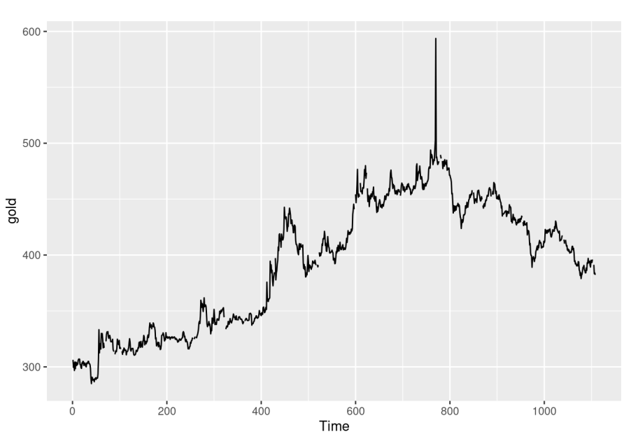
Now some markets have similarities. Those closer to gold mines are less impacted by shipping costs, so they show lower volatility in supply. Conversely, areas with wealthy buyers show less fluctuation in demand.
Our method will group similar time series’ together so our models can fit specialize and thereby exhibit higher accuracy.
2.1— Data Preprocessing
Data preprocessing is a manual process that helps derive signal out of potentially noisy and sparse data. A common first step is to remove outliers.
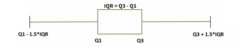
Tons of methods exist for non-temporal outlier detection, such as the classic IQR method (figure 3) where we exclude data that are sufficiently far from the center of our distribution. However, for time series data, we must take special precautions.
For instance, if there’s a strong trend, change in variance, or some other systematic change in our data over time, traditional outlier detection methods are invalidated.
To combat temporal changes in our data, we propose using an R package called tsclean. Fortunately it also supports missing data imputation, so if your time series has null values, you can easily interpolate them. After this step, we will have an uninterrupted time series with outliers removed, as shown in figure 4.
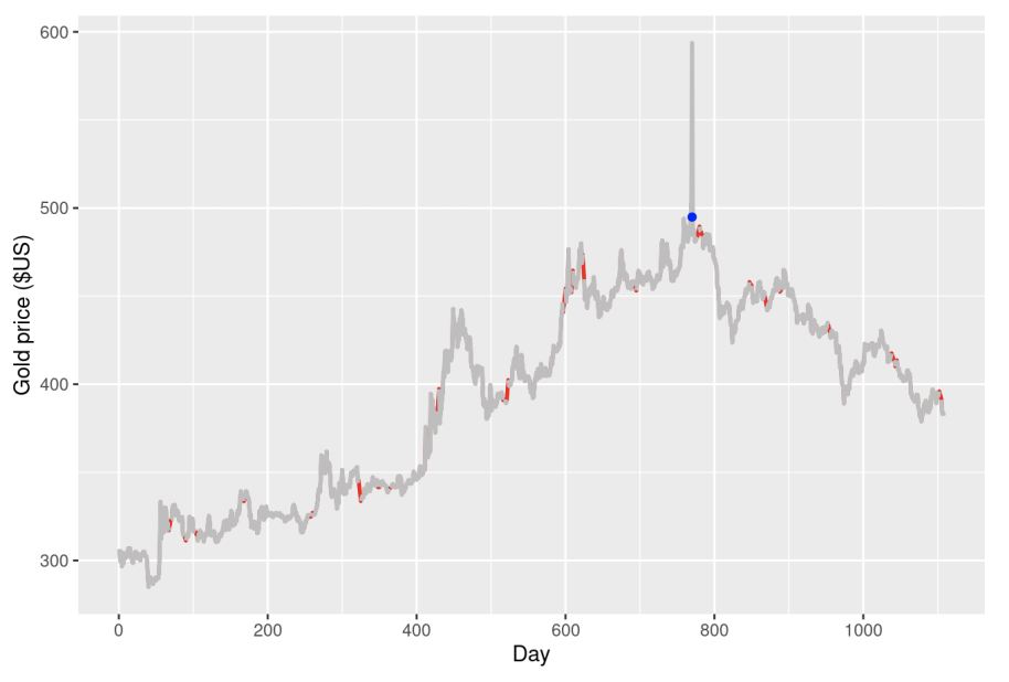
If you’re curious how the method works, in short, tsclean decomposes our time series into trend, seasonal, and “the rest” components, as show below.
From here, we use the IQR outlier detection method on R_t. By looking for outliers on a stationary (detrended) component of our time series, we’re more likely to find actual outliers instead of time-dependent changes.
Finally, as noted earlier, the tsclean package supports linear interpolation for data imputation. Linear interpolation simply replaces the missing values with the average of non-null points next to our missing value. Despite this functionality, the authors suggest using a different method called kNNImpute — R package. Unfortunately, kNNImpute is out of the scope of this post, however the above link provides a robust walkthrough.
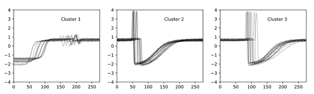
2.2 — Clustering
Now that we have a cleaned time series, we will cluster our time series values into similar sets.
The purpose of clustering is to improve accuracy of our models. By working with groups of similar data points, we are more likely to accurately fit the data.
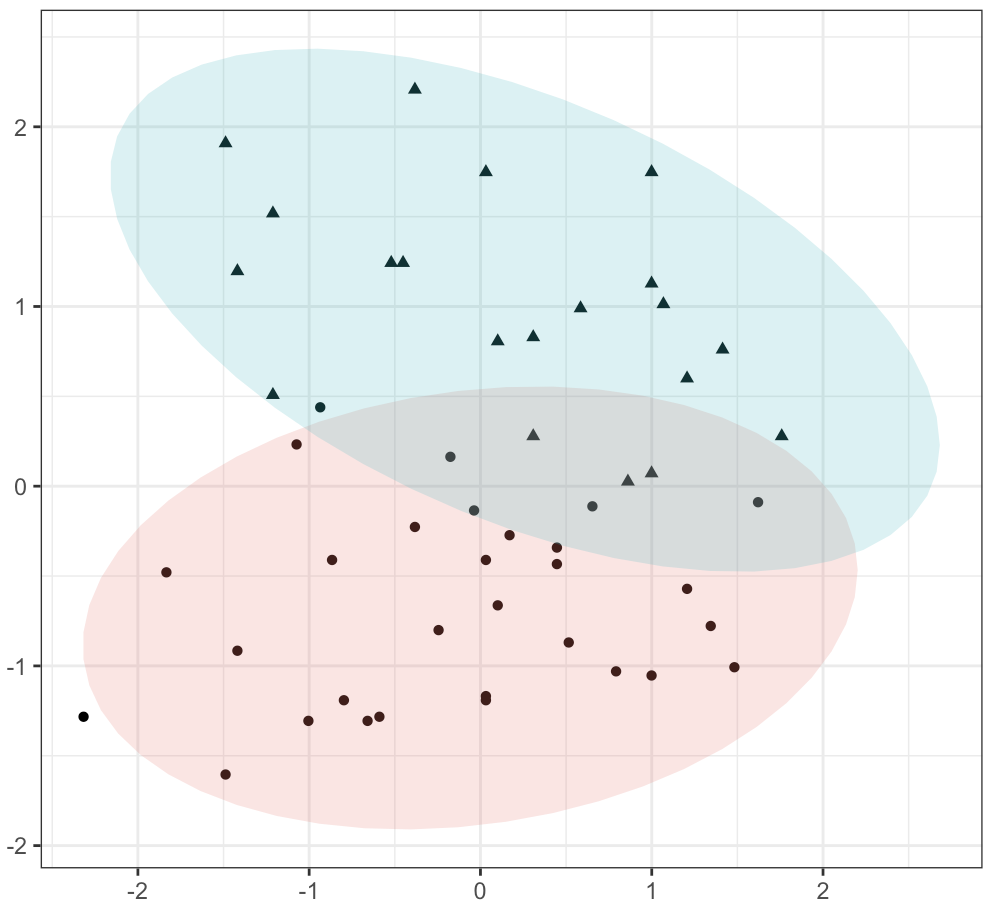
There are two broad types of clustering. The first type is called distance-based clustering. This is method simply looks to minimize the distance between data points within a cluster. The authors suggest using Dynamic Time Warping (DTW), which is a very robust and common measure of distance for sequential data. As with kNNImpute, this method is out of the scope of this post, but in short it adds constraints to the distance minimization goal to allow for more robust comparisons between sequential series’.
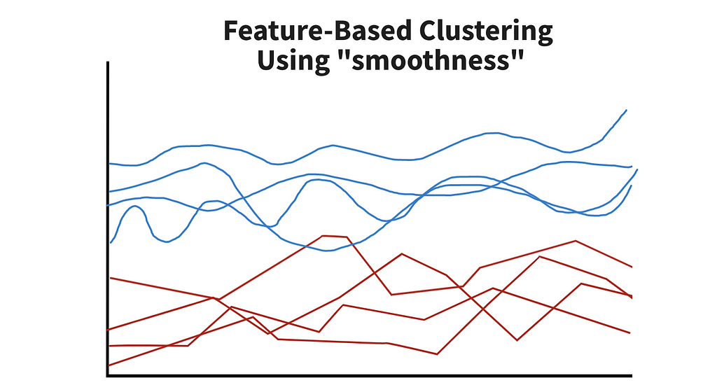
The second method is called feature-based clustering. As you’d expect, it uses features to group data points into different clusters. This can be hard to visualize, so we just created an example chart in figure 7.
In the paper, two sets of features were tested. The first included time-series-specific features, such as autocorrelation, partial autocorrelation, and the holt parameter. The second set borrowed ideas from signal processing and included energy, fast Fourier transform (FFT) coefficients, and variance. By leveraging information about the data, we would hopefully see patterns consistent within groups. From there, we can fit a model to each of the groups.
When run on simulated data, feature-based clustering outperformed distance-based clustering. And, of the two feature sets, signal-based features outperformed time series features.
2.3— Neural Network Architectures
Now that we have cleaned our original data and developed clusters, we are ready to develop our neural network architecture and train.
The paper outlines 7 architectures, some of which combined dynamic and static features. In our example of gold markets, a dynamic feature could be the weather and a static feature could be the location of the market.
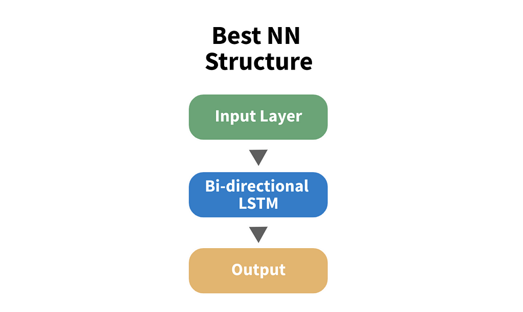
On the synthetic data tested in the paper, a simple bidirectional LSTM performed best. Surprisingly, static features in the synthetic data did not improve accuracy, however this observation is very data-dependent. For your use-case, you many want to explore other architectures that include static features.
And there you have it!
3 — Summary
In this post we covered how to preprocess and cluster time series data. Clustering alone was cited to improve classification accuracy by ~33%. However, it’s important to note that these tests were run on synthetic data — your data could see different levels of improvement.
To recap, we first preprocessed the data by removing outliers using seasonal decomposition paired with the IQR method. We then imputed missing data using K-nearest neighbors.
With a clean dataset, we clustered our time series data set. The most robust method involved using signal processing features.
From there, a bidirectional LSTM was the most effective method for the observed training data. Static features did not improve accuracy.
There are many alternatives discussed in the paper — if you need to improve model accuracy, it may be worth exploring those options.
Thanks for reading! I’ll be writing 31 more posts that bring academic research to the DS industry. Check out my comment for links to the main source for this post and some useful resources.
How to Improve Deep Learning Forecasts for Time Series was originally published in Towards Data Science on Medium, where people are continuing the conversation by highlighting and responding to this story.
from Towards Data Science - Medium https://ift.tt/3E20qNE
via RiYo Analytics


No comments