https://ift.tt/iZD0s7l What to look out for when moving to the all-new “ Compiled Mode” Photo by Mohamed Nohassi on Unsplash by Auth...
What to look out for when moving to the all-new “Compiled Mode”

Any new release of an AI development framework, AI accelerator, or AI computing platform, brings with it the potential for runtime optimization and cost reduction in our AI development life-cycle. The recent release of PyTorch 2.0 is no exception. Highlighted by the introduction of torch.compile, PyTorch 2.x can, reportedly, enable significant speedups for both training and inference. Contrary to the all-familiar PyTorch eager execution mode in which each PyTorch operation is run “eagerly”, the compile API converts your model into an intermediate computation graph (an FX graph) which it then compiles into low-level compute kernels in a manner that is optimal for the underlying training accelerator, using techniques such as kernel fusion and out-of-order execution (see here for more details).
In this post we will demonstrate the use of this exciting new feature as well as some of the issues and behaviors you might encounter when using it. You may have already come across some posts that highlight how easy it is to use torch compilation or how much it improves performance. Or (like me), you may have spent the last two weeks grappling with the new API trying to get it to work and perform well on your model. Indeed, for many public models all that is required is to wrap them with a torch.compile call (as reported here). However, as we will see, there are a number of things that can interfere with graph compilation and/or with reaching the desired performance improvement. Adapting your models and/or succeeding to reach optimal performance might require you to redesign your project or modify some of your coding habits.
A few things we should mention before we get started. Our intention in this post is to share just a few examples of the issues that we encountered while adapting the torch.compile API. The examples we will share are by no means comprehensive. It is very possible that you might run into an issue not mentioned here. Also keep in mind that torch.compile is still under active development. Some of the stuff we write might no longer be relevant by the time you read this. Be sure to stay up to date with the latest releases and documentation.
There are a number of innovative technologies underlying torch compilation, including TorchDynamo, FX Graph, TorchInductor, Triton, and more. While we will not dive into the different components in this post, we encourage you to learn about them from the PyTorch documentation, from the 2022 PyTorch conference, or from this helpful hands-on TDS post. Often times, a good understanding of what is happening behind the scenes can help you figure out why your model is not compiling and what you can do to fix it.
This post should not — in any way — be viewed as a replacement for the official PyTorch documentation (e.g., here). This post should also not be viewed as an endorsement for PyTorch over TensorFlow (or other ML training framework), for compile mode over eager mode, or for any other tool, library, or platform we should mention. I have found that all frameworks have their strengths and weaknesses. I do not have a strong preference or passion for any particular one. My passions lie in solving interesting technical challenges — the harder the better — regardless of the platform or framework upon which they reside. You could say that I am framework agnostic. All the same, allow me to indulge in two completely unimportant observations on how the PyTorch and TensorFlow libraries have evolved over time. Feel free to skip ahead to get back to the real stuff.
Two Completely Unimportant Observations on the TensorFlow vs. PyTorch Wars
Observation 1: In the olden days, when life was simple, there was a clear distinction between PyTorch and TensorFlow. PyTorch used eager execution mode, TensorFlow used graph mode, and everyone was happy because we all knew what we were fighting about. But then came TensorFlow 2 that introduced eager execution as the default execution mode and TensorFlow became a little bit more like PyTorch. And now PyTorch has come along, introduced its own graph compilation solution and become a little bit more like TensorFlow. The TensorFlow vs. PyTorch wars continue, but the differences between the two are slowly disappearing. See this tweet for one commentary on the PyTorch evolution that I found interesting.
Observation 2: AI development is a trendy business. Not unlike the fashion industry, the popular AI models, model architectures, learning algorithms, training frameworks, etc., change from season to season. Not unlike the fashion industry, AI has its own publications and conventions during which you can keep up with the latest trends. Until a few years ago, most of the models we worked on were written in TensorFlow. And people were unhappy. Their two primary complaints were that the high-level model.fit API limited their development flexibility and that graph mode made it impossible for them to debug. “We have to move to PyTorch”, they said, “where we can build our models any way we want and debug them easily". Fast forward a few years and the same folks are now saying “we have to adapt PyTorch Lightening (or some other high-level API) and we must speed up our training with torch.compile”. Just to be clear... I’m not judging. All I’m saying is that maybe we should be a bit more self-aware.
Back to the Real Stuff
The rest of the post is organized as a collection of tips for getting started with the PyTorch 2 compile API as well as some of the potential issues you might face. Depending on the specific details of your project, adapting your model to PyTorch’s graph mode may require a non-trivial effort. Our hope is that this post will help you better assess this effort and decide on the best way to take this step.
Installing PyTorch 2
From the PyTorch installation documentation, it would seem that installing PyTorch 2 is no different than installing any other PyTorch version. In practice there are some issues you may encounter. For one, PyTorch 2.0 appears (as of the time of this writing) to require Python version 3.8 or higher (see here). Hopefully, you are already up to date with one of the latest Python versions and this will not pose a problem for you, but in the unlikely (and unfortunate) case that you are not, this might be one more motivation for you to upgrade. Furthermore, PyTorch 2 contains package dependencies (most notably pytorch-triton) that did not exist in previous versions and may introduce new conflicts. To add to that, even if you succeed in building a PyTorch 2 environment, you might find that calling torch.compile results in a crushing and wholly unexplained segmentation fault.
One way to save yourself a lot of trouble is to take a pre-built and pre-validated PyTorch 2.0 Docker image. In the examples below, we will use an official AWS Deep Learning Container with PyTorch 2.0. Specifically, we will use the 763104351884.dkr.ecr.us-east-1.amazonaws.com/pytorch-training:2.0.0-gpu-py310-cu118-ubuntu20.04-sagemaker image designed for training on a GPU instance in Amazon SageMaker with Python 3.10 and PyTorch 2.0.
Backward Compatibility
One of the nice things about PyTorch 2 is that it is fully backward compatible. Thus, even if you choose to stick with eager execution mode and not use torch.compile at this time, you are still highly encouraged to upgrade to PyTorch 2.0 and benefit from the other new features and enhancements.
Toy Example
Let’s jump right in with a toy example of an image classification model. In the following code block we build a basic Vision Transformer (ViT) model using the timm Python package (version 0.6.12) and train it on a fake dataset for 500 steps. We define the use_compile flag to control whether to perform model compilation (torch.compile) and the use_amp to control whether to run using Automatic Mixed Precision (AMP) or full precision (FP).
import time, os
import torch
from torch.utils.data import Dataset
from timm.models.vision_transformer import VisionTransformer

use_amp = True # toggle to enable/disable amp
use_compile = True # toggle to use eager/graph execution mode

# use a fake dataset (random data)
class FakeDataset(Dataset):
  def __len__(self):
    return 1000000

  def __getitem__(self, index):
    rand_image = torch.randn([3, 224, 224], dtype=torch.float32)
    label = torch.tensor(data=[index % 1000], dtype=torch.int64)
    return rand_image, label

def train():
  device = torch.cuda.current_device()
  dataset = FakeDataset()
  batch_size = 64

  # define an image classification model with a ViT backbone
  model = VisionTransformer()

  if use_compile:
    model = torch.compile(model)

  model.to(device)

  optimizer = torch.optim.Adam(model.parameters())
  data_loader = torch.utils.data.DataLoader(dataset,
                          batch_size=batch_size, num_workers=4)
  loss_function = torch.nn.CrossEntropyLoss()

  t0 = time.perf_counter()
  summ = 0
  count = 0

  for idx, (inputs, target) in enumerate(data_loader, start=1):
    inputs = inputs.to(device)
    targets = torch.squeeze(target.to(device), -1)

    optimizer.zero_grad()

    with torch.cuda.amp.autocast(
      enabled=use_amp,
      dtype=torch.bfloat16
    ):
      outputs = model(inputs)
      loss = loss_function(outputs, targets)

    loss.backward()
    optimizer.step()

    batch_time = time.perf_counter() - t0

    if idx > 10:  # skip first few steps
      summ += batch_time
      count += 1
    t0 = time.perf_counter()
    if idx > 500:
      break

  print(f'average step time: {summ/count}')

if __name__ == '__main__':
  train()
In the table below we demonstrate the comparative performance results when running the training script on an ml.g5.xlarge instance type using Amazon SageMaker. The impact of model compilation will differ from platform to platform (e.g., see here). Generally speaking the speed-up will be higher on more modern server-class GPUs. Keep in mind that these are just examples of the types of results that you might see. The actual results will be highly dependent on the specific details of your project.

We can see that the performance boost from model compilation is far more pronounced when using AMP (28.6%) than when using FP (4.5%). This is a well-known discrepancy (e.g., see here). If you don’t already train with AMP, you might find that the most significant performance gain can be achieved by transitioning from FP to AMP. We can also see that in the case of our model, the performance boost came with a very slight increase in GPU memory utilization.
Note that the comparative performance might change when scaling to multiple GPUs due to the way in which distributed training is implemented on compiled graphs. See here for more details.
Advanced Compilation Options
The torch.compile API includes a number of options for controlling the graph creation. These enable you to fine-tune the compilation for your specific model and potentially boost performance even more. The code block below contains the function signature (from this source).
def compile(model: Optional[Callable] = None, *,
            fullgraph: builtins.bool = False,
            dynamic: builtins.bool = False,
            backend: Union[str, Callable] = "inductor",
            mode: Union[str, None] = None,
            options: Optional[Dict[str, Union[str, builtins.int, builtins.bool]]] = None,
            disable: builtins.bool = False) -> Callable:
    """
    Optimizes given model/function using TorchDynamo and specified backend.

    Args:
       model (Callable): Module/function to optimize
       fullgraph (bool): Whether it is ok to break model into several subgraphs
       dynamic (bool): Use dynamic shape tracing
       backend (str or Callable): backend to be used
       mode (str): Can be either "default", "reduce-overhead" or "max-autotune"
       options (dict): A dictionary of options to pass to the backend.
       disable (bool): Turn torch.compile() into a no-op for testing
    """
Compilation Mode: The compilation mode allows you to choose between minimizing the overhead required by compilation (“reduce-overhead”) and maximizing potential performance boost (“max-autotune”). See here for more details.
In the table below we compare the results of compiling the ViT model above with different compilation modes.
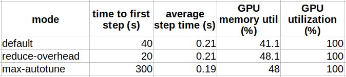
We can see that the compilation modes behave pretty much as advertised, with “reduce-overhead” reducing the compilation time at the cost of extra memory utilization and “max-autotune” resulting in maximum performance at the expense of high overhead in compilation time.
Compiler Backend: The compile API allows you determine which backend to use to convert the intermediate representation (IR) computation graph (the FX graph) into low-level kernel operations. This option is useful for debugging graph compilation issues and for gaining a better understanding for the torch.compile internals (as demonstrated in this cool example). In most cases (as of the time of this writing) the default, TorchInductor backend, appears to provide the best training performance results. See here for the current list of existing backends, or run the code below to see the ones that are supported in your environment. And if you really want, you can also add your own backend :).
from torch import _dynamo
print(_dynamo.list_backends())
For example, by modifying the code above to use the nvprims-nvfuser backend we get an 13% performance boost over eager mode (compared to the 28.6% boost with the default backend).
Force a Single Graph: The fullgraph flag is an extremely useful control for ensuring that you do not have any undesired graph-breaks. More on this topic below.
Dynamic Shape Flag: As of the time of this writing, compilation support for tensors that have dynamic shapes is somewhat limited. A common byproduct of compiling a model with dynamic shapes is excessive recompilation which can significantly increase overhead and slow your training down considerably. If your model does include dynamic shapes, setting the dynamic flag to True will result in better performance and, in particular, reduce the number of recompilations.
Performance Profiling
We have written extensively (e.g., here) about the importance of profiling the training performance as a means to accelerating training speed and reducing cost. One of the key tools we use for profiling performance of PyTorch models is the PyTorch Profiler. The PyTorch profiler allows us to assess and analyze the manner in which graph compilation optimizes the training step. In the code block below we wrap our training loop with a torch.profiler and generate the results for TensorBoard. We save the output in the SM_MODEL_DIR which is automatically uploaded to persistent storage at the end of the training job.
  out_path = os.path.join(os.environ.get('SM_MODEL_DIR','/tmp'),'profile')
  from torch.profiler import profile, ProfilerActivity
  with profile(
          activities=[ProfilerActivity.CPU, ProfilerActivity.CUDA],
          schedule=torch.profiler.schedule(
            wait=20,
            warmup=5,
            active=10,
            repeat=1),
          on_trace_ready=torch.profiler.tensorboard_trace_handler(
                                                dir_name=out_path)

  ) as p:
    for idx, (inputs, target) in enumerate(data_loader, start=1):
      inputs = inputs.to(device)
      targets = torch.squeeze(target.to(device), -1)
      optimizer.zero_grad()

      with torch.cuda.amp.autocast(
        enabled=use_amp,
        dtype=torch.bfloat16
      ):
        outputs = model(inputs)
        loss = loss_function(outputs, targets)
      loss.backward()
      optimizer.step()
      p.step()
The image below was captured from the GPU Kernel view of the TensorBoard PyTorch Profiler tab. It provides details of the kernels that are run on the GPU during the training step of the compiled model trial from above.
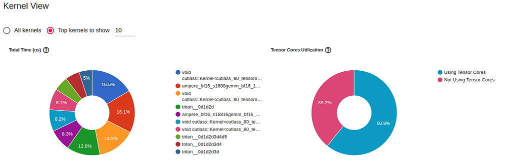
By comparing these charts to the ones from the eager execution run, we are able to see that graph compilation increases the utilization of the GPU’s Tensor Cores (from 51% to 60%) and that it introduces the use of GPU kernels developed using Triton.
Diagnosing Model Compilation Issues
PyTorch compilation is still under active development (currently in beta) and it is not at all unlikely that you will encounter issues when compiling your model. If you are lucky, you will get an informative error and will have an easy (and reasonable) way to work around it. If you are less lucky, you may have to work a bit harder to find the root of the issue, and/or may come to the conclusion that, at its current maturity level, model compilation does not address your needs.
The primary resource for addressing compilation issues is the TorchDynamo troubleshooting page which includes a list of debugging tools and offers a step-by-step guide for diagnosing errors. Unfortunately, as of the time of this writing, the tools and techniques appear to be targeted more towards PyTorch developers than PyTorch users. They can be helpful in root-causing compilation issues, providing some hints as to how you might be able to work around them, and/or reporting them to PyTorch. However, you might find that they don’t help in actually resolving your issues.
In the code block below we show a simple distributed model that includes a call to torch.distributed.all_reduce. This model runs as expected in eager mode, but fails (as of the time of this writing) with an “attribute error” during graph compilation (torch.classes.c10d.ProcessGroup does not have a field with name ‘shape’). By increasing the log level to INFO we find that the error is in “step #3” of the calculation, the TorchInductor. We can confirm this by verifying that compilation succeeds with the “eager” and “aot_eager” backends. Finally, we can create a minimal code sample that reproduces the failure using the PyTorch Minifier.
import os, logging
import torch
from torch import _dynamo

# enable debug prints
torch._dynamo.config.log_level = logging.INFO
torch._dynamo.config.verbose=True

# uncomment to run minifier
# torch._dynamo.config.repro_after="aot"

def build_model():
  import torch.nn as nn
  import torch.nn.functional as F

  class DumbNet(nn.Module):
    def __init__(self):
      super().__init__()
      self.conv1 = nn.Conv2d(3, 6, 5)
      self.pool = nn.MaxPool2d(2, 2)
      self.fc1 = nn.Linear(1176, 10)

    def forward(self, x):
      x = self.pool(F.relu(self.conv1(x)))
      x = torch.flatten(x, 1)
      x = self.fc1(x)
      with torch.no_grad():
        sum_vals = torch.sum(x,0)
        # this is the problematic line of code
        torch.distributed.all_reduce(sum_vals)
      # add noise
      x = x + 0.1*sum_vals
      return x

  net = DumbNet()
  return net

def train():
  os.environ['MASTER_ADDR'] = os.environ.get('MASTER_ADDR',
                                             'localhost')
  os.environ['MASTER_PORT'] = os.environ.get('MASTER_PORT',
                                             str(2222))
  torch.distributed.init_process_group('nccl', rank=0,
                                         world_size=1)
  torch.cuda.set_device(0)
  device = torch.cuda.current_device()

  model = build_model()

  model = torch.compile(model)

  # replace with this to verfiy that error is not in TorchDynamo
  # model = torch.compile(model, 'eager')
  # replace with this to verfiy that error is not in AOTAutograd
  # model = torch.compile(model, 'aot_eager')

  model.to(device)

  rand_image = torch.randn([4, 3, 32, 32], dtype=torch.float32).to(device)

  model(rand_image)

if __name__ == '__main__':
  train()
Sadly, in our example, running the generated minifier_launcher.py script results in a different attribute error (‘Repro’ object has no attribute ‘_tensor_constant0’), and despite having enjoyed the whole experience, the documented debugging steps did not help all that much in solving the compilation issue we demonstrated.
Obviously, we hope that you do not run into any compilation issues. In case you do, know that: 1. you are not alone :), and 2. although they are likely to be different than the one demonstrated here, following the same steps described in the troubleshooting guide may give some indication as to their source.
Common Graph Breaks
One of the most touted advantages of Pytorch eager mode is the ability to interleave pure Pythonic code with your PyTorch operations. Unfortunately, this freedom (as of the time of this writing) is significantly restricted when using torch.compile. The reason for this is that certain Pythonic operations cause TorchDynamo to split the computation graph into multiple components, thus hindering the potential for performance gains. Your goal should be to minimize such graph breaks to the extent possible. As a best practice, you might consider compiling your model with the fullgraph flag when you are porting your model to PyTorch 2. Not only will this encourage you to remove any code that causes graph breaks, but it will also teach you how to best adapt your PyTorch development habits for using graph mode. However, note that you will have to disable this flag to run distributed code as the current way that communication between GPUs is implemented requires graph breaks (e.g., see here). Alternatively, you can use the torch._dynamo.explain utility to analyze graph breaks, as described here.
The following code block demonstrates a simple model with four potential graph breaks in its forward pass (as of the time of this writing). It is not uncommon to see any one of these kinds of operations in a typical PyTorch model.
import torch
from torch import _dynamo
import numpy as np

def build_model():
  import torch.nn as nn
  import torch.nn.functional as F

  class DumbNet(nn.Module):
    def __init__(self):
      super().__init__()
      self.conv1 = nn.Conv2d(3, 6, 5)
      self.pool = nn.MaxPool2d(2, 2)
      self.fc1 = nn.Linear(1176, 10)
      self.fc2 = nn.Linear(10, 10)
      self.fc3 = nn.Linear(10, 10)
      self.fc4 = nn.Linear(10, 10)
      self.d = {}


    def forward(self, x):
      x = self.pool(F.relu(self.conv1(x)))
      x = torch.flatten(x, 1)
      assert torch.all(x >= 0) # graph break
      x = self.fc1(x)
      self.d['fc1-out'] = x.sum().item() # graph break
      x = self.fc2(x)
      for k in np.arange(1): # graph break
        x = self.fc3(x)
      print(x)  # graph break
      x = self.fc4(x)
      return x

  net = DumbNet()
  return net

def train():
  model = build_model()
  rand_image = torch.randn([4, 3, 32, 32], dtype=torch.float32)
  explanation = torch._dynamo.explain(model, rand_image)
  print(explanation)

if __name__ == '__main__':
  train()
It is important to emphasize that graph breaks do not fail the compilation (unless the fullgraph flag is set). Thus, it is perfectly possible that your model is compiling and running but actually contains multiple graph breaks that are slowing it down.
Troubleshooting Training Issues
While succeeding in compiling your model is a worthy achievement, it is not a guarantee that training will succeed. As noted above, the low-level kernels that run on the GPU will differ between eager mode and graph mode. Consequently, certain high-level operations may exhibit different behaviors. In particular, you might find that operations that run in eager mode fail in graph mode (e.g., this torch.argmin failure that we encountered). Alternatively, you might find that numerical differences in computation have an impact on your training.
To make matters worse, debugging in graph mode is much more difficult than in eager mode. In eager mode each line of code is executed independently, allowing us to place a breakpoint at any point in our code and evaluate the current tensor values. In graph mode, on the other hand, the model defined by our code undergoes multiple transitions before being processed and, consequently, your breakpoint may not be triggered.
In the past, we expanded on the difficulties of debugging in graph mode in TensorFlow and proposed a few ways to address them. Here is a two-step approach you could try when you encounter an issue. First, revert back to eager mode where debugging is less difficult and pray that the issue reproduces. If it does not, evaluate intermediate tensors of interest in your compiled computation graph by purposely inserting graph breaks in your model. You can do this by either explicitly breaking your model into two (or more) portions and applying torch.compile to each portion separately, or by generating a graph break by inserting a print, and/or a Tensor.numpy invocation as described in the previous section. Depending on how you do this, you may even succeed in triggering breakpoints in your code. Still, keep in mind that breaking up your graph in this manner can modify the sequence of low-level operations so it may not accurately reproduce the fully compiled graph execution. But it certainly gives you more flexibility in trying to get to the bottom of your issue.
See the accuracy-debugging portion of the troubleshooting guide if you encounter discrepancies between compile mode and eager mode that are unexpected.
Including the Loss Function in the Graph
As we demonstrated in the examples above, graph execution mode is enabled by wrapping a PyTorch model (or function) with a torch.compile invocation. You may have observed that the loss function is not part of the compilation call and, as a result, not part of the generated graph. In many cases, including the ones that we have demonstrated, the loss function is a relatively small portion of the training step and running it eagerly will not incur much overhead. However, if you have a particularly heavy loss you may be able to further boost performance by including it in the compiled computation graph. For example, in the code block below, we define a loss function for (naively) performing model distillation from a large ViT model (with 24 ViT blocks) to a smaller ViT model (with 12 ViT blocks).
import torch
from timm.models.vision_transformer import VisionTransformer

class ExpensiveLoss(torch.nn.Module):
  def __init__(self):
    super(ExpensiveLoss, self).__init__()
    self.expert_model = VisionTransformer(depth=24)
    if torch.cuda.is_available():
      self.expert_model.to(torch.cuda.current_device())
    self.mse_loss = torch.nn.MSELoss()

  def forward(self, input, outputs):
    expert_output = self.expert_model(input)
    return self.mse_loss(outputs, expert_output)
Our implementation includes a loss function that calls the large model on each input batch. This is a much more compute-heavy loss function than the CrossEntropyLoss above and running it eagerly would not be ideal.
We describe two ways to solve this. The first is to simply wrap the loss function in a torch.compile invocation of its own, as shown here:
loss_function = ExpensiveLoss()
compiled_loss = torch.compile(loss_function)
The disadvantage of this option is that the compiled graph of the loss function is disjoint from the compiled graph of the model. The second option compiles the model and loss together by creating a wrapper model that includes both and returns the resultant loss as its output. This option is demonstrated in the code block below:
import time, os
import torch
from torch.utils.data import Dataset
from torch import nn
from timm.models.vision_transformer import VisionTransformer

# use a fake dataset (random data)
class FakeDataset(Dataset):
  def __len__(self):
    return 1000000

  def __getitem__(self, index):
    rand_image = torch.randn([3, 224, 224], dtype=torch.float32)
    label = torch.tensor(data=[index % 1000], dtype=torch.int64)
    return rand_image, label

# create a wrapper model for the ViT model and loss
class SuperModel(torch.nn.Module):
  def __init__(self):
    super(SuperModel, self).__init__()
    self.model = VisionTransformer()
    self.expert_model = VisionTransformer(depth=24 if torch.cuda.is_available() else 2)
    self.mse_loss = torch.nn.MSELoss()

  def forward(self, inputs):
    outputs = self.model(inputs)
    with torch.no_grad():
      expert_output = self.expert_model(inputs)
    return self.mse_loss(outputs, expert_output)

# a loss that simply passes through the model output
class PassthroughLoss(nn.Module):
  def __call__(self, model_output):
    return model_output

def train():
  device = torch.cuda.current_device()
  dataset = FakeDataset()
  batch_size = 64

  # create and compile the model
  model = SuperModel()
  model = torch.compile(model)

  model.to(device)

  optimizer = torch.optim.Adam(model.parameters())
  data_loader = torch.utils.data.DataLoader(dataset,
                          batch_size=batch_size, num_workers=4)

  loss_function = PassthroughLoss()

  t0 = time.perf_counter()
  summ = 0
  count = 0

  for idx, (inputs, target) in enumerate(data_loader, start=1):
    inputs = inputs.to(device)
    targets = torch.squeeze(target.to(device), -1)

    optimizer.zero_grad()

    with torch.cuda.amp.autocast(
      enabled=True,
      dtype=torch.bfloat16
    ):
      outputs = model(inputs)
      loss = loss_function(outputs)

    loss.backward()
    optimizer.step()

    batch_time = time.perf_counter() - t0

    if idx > 10:  # skip first few steps
      summ += batch_time
      count += 1
    t0 = time.perf_counter()
    if idx > 500:
      break

  print(f'average step time: {summ/count}')

if __name__ == '__main__':
  train()
The disadvantage of this approach is that the internal model will need to be extracted from the wrapper model when the time comes to run the model in inference mode.
In our case, both options result in roughly the same 8% performance boost, demonstrating the importance of this kind of optimization. When the loss is run eagerly, the total step time is 0.37 seconds, and when the loss is compiled, the total step time is 0.34 seconds.
Dynamic Shapes
As reported in the documentation, compilation support for models with dynamic shapes is limited (as of the time of this writing). Depending on the details of the dynamism, dynamic models could incur significant performance overhead, either by introducing graph breaks and/or triggering an excessive number of graph recompilations. Graph recompilations occur when one of the assumptions (referred to as guards) about the model that were made during the original compilation is violated.
The torch.compile API includes the dynamic flag for signaling to the compiler to optimize for dynamic shapes. However, as of the time of this writing, the degree to which this will help is questionable. If you are trying to compile and optimize a dynamic graph and facing issues, you might choose to hold off on this until the level of support matures.
Summary
PyTorch 2.0 compile mode comes with the potential for a considerable boost to the speed of training and inference and, consequently, meaningful savings in cost. However, the amount of work that your model will require to realize this potential can vary greatly. Many public models require nothing more than changing a single line of code. Other models, especially ones that include non-standard operations, dynamic shapes, and/or a lot of interleaved Python code, might require more considerable effort. However, there may be no better time to start adapting your models than today, as it appears that compile mode is here to stay.
Tips and Tricks for Upgrading to PyTorch 2.0 was originally published in Towards Data Science on Medium, where people are continuing the conversation by highlighting and responding to this story.
from Towards Data Science - Medium
https://towardsdatascience.com/tips-and-tricks-for-upgrading-to-pytorch-2-3127db1d1f3d?source=rss----7f60cf5620c9---4
via RiYo Analytics


No comments