https://ift.tt/WuO0tVj Using gradients to understand how your model predicts Image by author. X-ray image from the kaggle chest X-ray dat...
Using gradients to understand how your model predicts
I took notice of a technique called Grad-CAM that enables the inspection of how a convolutional neural network predicts its outputs. For example, in a classifier, you can gain insight into how your neural network used the input to make its prediction. It all started with the original paper that described it. In this article, we’re going to implement it using the Pytorch library in a way that you can apply to any convolutional neural network without needing to change anything in the neural network module you already have.
I read a paper here on Medium called “Implementing Grad-CAM in PyTorch,” by Stepan Ulyanin, which inspired me to implement the same algorithm in a slightly different way. Stepan proposed an approach that requires you to rewrite the forward function of your model to compute Grad-CAM. Thanks to Pytorch, we can achieve the same result without changing the forward function by registering forward and backward hooks. I hope this article contributes a little to the amazing work that Stepan wrote.
Let’s dive into it!
1. Load and inspect the pre-trained model
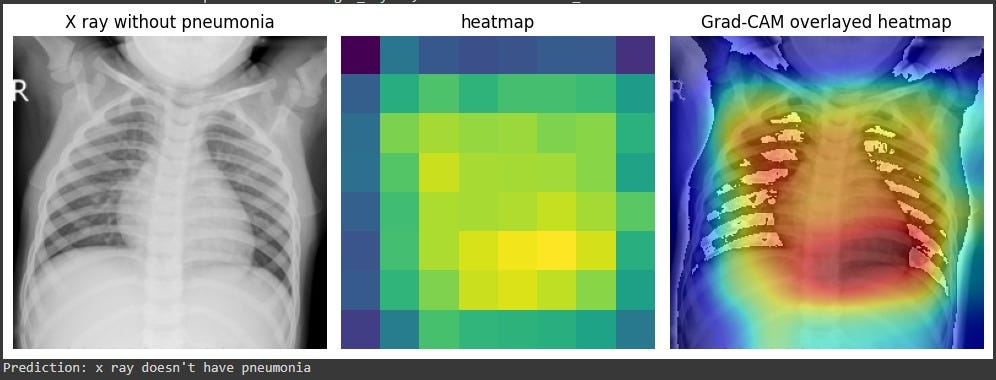
To demonstrate the implementation of Grad-CAM, I’ll use a chest X-ray dataset from Kaggle and a pre-trained classifier I made, capable of classifying an X-ray as having pneumonia or not.
model_path = "your/model/path/"

# instantiate your model
model = XRayClassifier()

# load your model. Here we're loading on CPU since we're not going to do
# large amounts of inference
model.load_state_dict(torch.load(model_path, map_location=torch.device('cpu')))

# put it in evaluation mode for inference
model.eval()
Next, let’s inspect the model’s architecture. Since we are interested in understanding which aspects of our input image contributed to the prediction, we need to identify the last convolutional layer, specifically its activation function. This layer contains the representation of the most complex features the model learned to classify its inputs. Thus, it is the most capable of helping us understand the model’s behavior.
import torch
import torch.nn as nn
import torch.nn.functional as F

# hyperparameters
nc = 3 # number of channels
nf = 64 # number of features to begin with
dropout = 0.2
device = torch.device('cuda' if torch.cuda.is_available() else 'cpu')

# setup a resnet block and its forward function
class ResNetBlock(nn.Module):
    def __init__(self, in_channels, out_channels, stride=1):
        super(ResNetBlock, self).__init__()
        self.conv1 = nn.Conv2d(in_channels, out_channels, kernel_size=3, stride=stride, padding=1, bias=False)
        self.bn1 = nn.BatchNorm2d(out_channels)
        self.conv2 = nn.Conv2d(out_channels, out_channels, kernel_size=3, stride=1, padding=1, bias=False)
        self.bn2 = nn.BatchNorm2d(out_channels)

        self.shortcut = nn.Sequential()
        if stride != 1 or in_channels != out_channels:
            self.shortcut = nn.Sequential(
                nn.Conv2d(in_channels, out_channels, kernel_size=1, stride=stride, bias=False),
                nn.BatchNorm2d(out_channels)
            )

    def forward(self, x):
        out = F.relu(self.bn1(self.conv1(x)))
        out = self.bn2(self.conv2(out))
        out += self.shortcut(x)
        out = F.relu(out)
        return out

# setup the final model structure
class XRayClassifier(nn.Module):
    def __init__(self, nc=nc, nf=nf, dropout=dropout):
        super(XRayClassifier, self).__init__()

        self.resnet_blocks = nn.Sequential(
            ResNetBlock(nc,   nf,    stride=2), # (B, C, H, W) -> (B, NF, H/2, W/2), i.e., (64,64,128,128)
            ResNetBlock(nf,   nf*2,  stride=2), # (64,128,64,64)
            ResNetBlock(nf*2, nf*4,  stride=2), # (64,256,32,32)
            ResNetBlock(nf*4, nf*8,  stride=2), # (64,512,16,16)
            ResNetBlock(nf*8, nf*16, stride=2), # (64,1024,8,8)
        )

        self.classifier = nn.Sequential(
            nn.Conv2d(nf*16, 1, 8, 1, 0, bias=False),
            nn.Dropout(p=dropout),
            nn.Sigmoid(),
        )

    def forward(self, input):
        output = self.resnet_blocks(input.to(device))
        output = self.classifier(output)
        return output
This model was designed to receive 256x256 images with 3 channels. Therefore, its input is expected to have a shape of [batch size, 3, 256, 256]. Every ResNet block ends with a ReLU activation function. For our objective here, we need to select the last ResNet block.
XRayClassifier(
  (resnet_blocks): Sequential(
    (0): ResNetBlock(
      (conv1): Conv2d(3, 64, kernel_size=(3, 3), stride=(2, 2), padding=(1, 1), bias=False)
      (bn1): BatchNorm2d(64, eps=1e-05, momentum=0.1, affine=True, track_running_stats=True)
      (conv2): Conv2d(64, 64, kernel_size=(3, 3), stride=(1, 1), padding=(1, 1), bias=False)
      (bn2): BatchNorm2d(64, eps=1e-05, momentum=0.1, affine=True, track_running_stats=True)
      (shortcut): Sequential(
        (0): Conv2d(3, 64, kernel_size=(1, 1), stride=(2, 2), bias=False)
        (1): BatchNorm2d(64, eps=1e-05, momentum=0.1, affine=True, track_running_stats=True)
      )
    )
    (1): ResNetBlock(
      (conv1): Conv2d(64, 128, kernel_size=(3, 3), stride=(2, 2), padding=(1, 1), bias=False)
      (bn1): BatchNorm2d(128, eps=1e-05, momentum=0.1, affine=True, track_running_stats=True)
      (conv2): Conv2d(128, 128, kernel_size=(3, 3), stride=(1, 1), padding=(1, 1), bias=False)
      (bn2): BatchNorm2d(128, eps=1e-05, momentum=0.1, affine=True, track_running_stats=True)
      (shortcut): Sequential(
        (0): Conv2d(64, 128, kernel_size=(1, 1), stride=(2, 2), bias=False)
        (1): BatchNorm2d(128, eps=1e-05, momentum=0.1, affine=True, track_running_stats=True)
      )
    )
    (2): ResNetBlock(
      (conv1): Conv2d(128, 256, kernel_size=(3, 3), stride=(2, 2), padding=(1, 1), bias=False)
      (bn1): BatchNorm2d(256, eps=1e-05, momentum=0.1, affine=True, track_running_stats=True)
      (conv2): Conv2d(256, 256, kernel_size=(3, 3), stride=(1, 1), padding=(1, 1), bias=False)
      (bn2): BatchNorm2d(256, eps=1e-05, momentum=0.1, affine=True, track_running_stats=True)
      (shortcut): Sequential(
        (0): Conv2d(128, 256, kernel_size=(1, 1), stride=(2, 2), bias=False)
        (1): BatchNorm2d(256, eps=1e-05, momentum=0.1, affine=True, track_running_stats=True)
      )
    )
    (3): ResNetBlock(
      (conv1): Conv2d(256, 512, kernel_size=(3, 3), stride=(2, 2), padding=(1, 1), bias=False)
      (bn1): BatchNorm2d(512, eps=1e-05, momentum=0.1, affine=True, track_running_stats=True)
      (conv2): Conv2d(512, 512, kernel_size=(3, 3), stride=(1, 1), padding=(1, 1), bias=False)
      (bn2): BatchNorm2d(512, eps=1e-05, momentum=0.1, affine=True, track_running_stats=True)
      (shortcut): Sequential(
        (0): Conv2d(256, 512, kernel_size=(1, 1), stride=(2, 2), bias=False)
        (1): BatchNorm2d(512, eps=1e-05, momentum=0.1, affine=True, track_running_stats=True)
      )
    )
    (4): ResNetBlock(
      (conv1): Conv2d(512, 1024, kernel_size=(3, 3), stride=(2, 2), padding=(1, 1), bias=False)
      (bn1): BatchNorm2d(1024, eps=1e-05, momentum=0.1, affine=True, track_running_stats=True)
      (conv2): Conv2d(1024, 1024, kernel_size=(3, 3), stride=(1, 1), padding=(1, 1), bias=False)
      (bn2): BatchNorm2d(1024, eps=1e-05, momentum=0.1, affine=True, track_running_stats=True)
      (shortcut): Sequential(
        (0): Conv2d(512, 1024, kernel_size=(1, 1), stride=(2, 2), bias=False)
        (1): BatchNorm2d(1024, eps=1e-05, momentum=0.1, affine=True, track_running_stats=True)
      )
    )
  )
  (classifier): Sequential(
    (0): Conv2d(1024, 1, kernel_size=(8, 8), stride=(1, 1), bias=False)
    (1): Dropout(p=0.2, inplace=False)
    (2): Sigmoid()
  )
)
In Pytorch, we can make this selection quite easily using the model’s attributes.
model.resnet_blocks[-1]
#ResNetBlock(
#  (conv1): Conv2d(512, 1024, kernel_size=(3, 3), stride=(2, 2), padding=(1, 1), bias=False)
#  (bn1): BatchNorm2d(1024, eps=1e-05, momentum=0.1, affine=True, track_running_stats=True)
#  (conv2): Conv2d(1024, 1024, kernel_size=(3, 3), stride=(1, 1), padding=(1, 1), bias=False)
#  (bn2): BatchNorm2d(1024, eps=1e-05, momentum=0.1, affine=True, track_running_stats=True)
#  (shortcut): Sequential(
#    (0): Conv2d(512, 1024, kernel_size=(1, 1), stride=(2, 2), bias=False)
#    (1): BatchNorm2d(1024, eps=1e-05, momentum=0.1, affine=True, track_running_stats=True)
#  )
#)
2. Pytorch methods for registering hooks
Pytorch has many functions to handle hooks, which are functions that allow you to process information that flows through the model during the forward or backward pass. You can use it to inspect intermediate gradient values, make changes to specific layers’ outputs, and more.
Here, we’ll focus on two methods of the nn.Module class. Let’s have a closer look at them.
2.1. register_full_backward_hook(hook, prepend=False)
This method registers a backward hook on the module, which means that the hook function will run when the backward() method is called.
The backward hook function receives as inputs the module itself, the gradients with respect to the layer’s input, and the gradients with respect to the layer’s output.
hook(module, grad_input, grad_output) -> tuple(Tensor) or None
It returns a torch.utils.hooks.RemovableHandle, which allows you to remove the hook later. Therefore, it is useful to assign it to a variable. We’ll get back to this later.
2.2. register_forward_hook(hook, *, prepend=False, with_kwargs=False)
This is quite similar to the previous one, except that the hook function runs in the forward pass, i.e., when the layer of interest processes its input and returns its outputs.
The hook function has a slightly different signature. It gives you access to the layer’s outputs:
hook(module, args, output) -> None or modified output
It also returns a torch.utils.hooks.RemovableHandle.
3. Adding backward and forward hooks to your model
First, we need to define our backward and forward hook functions. To compute Grad-CAM, we need the gradients with respect to the last convolutional layer’s outputs, as well as its activations, i.e., the outputs of the layer’s activation function. Therefore, our hook functions will only extract those values for us during inference and the backward pass.
# defines two global scope variables to store our gradients and activations
gradients = None
activations = None

def backward_hook(module, grad_input, grad_output):
  global gradients # refers to the variable in the global scope
  print('Backward hook running...')
  gradients = grad_output
  # In this case, we expect it to be torch.Size([batch size, 1024, 8, 8])
  print(f'Gradients size: {gradients[0].size()}')
  # We need the 0 index because the tensor containing the gradients comes
  # inside a one element tuple.

def forward_hook(module, args, output):
  global activations # refers to the variable in the global scope
  print('Forward hook running...')
  activations = output
  # In this case, we expect it to be torch.Size([batch size, 1024, 8, 8])
  print(f'Activations size: {activations.size()}')
After defining our hook functions and the variables that will store the activations and the gradients, we need to register the hooks on the layer of interest:
backward_hook = model.resnet_blocks[-1].register_full_backward_hook(backward_hook, prepend=False)
forward_hook = model.resnet_blocks[-1].register_forward_hook(forward_hook, prepend=False)
4. Retrieving the gradients and activations we need
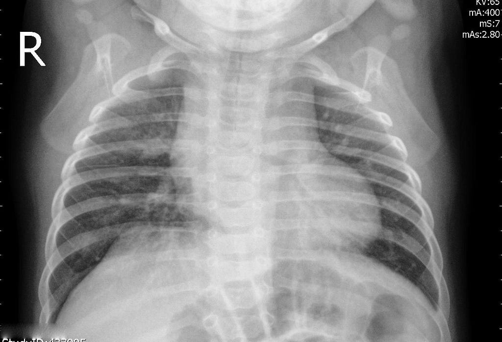
Now that we have set up the hooks for our model, let’s load an image for which we will compute Grad-CAM.
from PIL import Image

img_path = "/your/image/path/"
image = Image.open(img_path).convert('RGB')
We need to preprocess it to prepare it for being fed into the model for inference.
from torchvision import transforms
from torchvision.transforms import ToTensor

image_size = 256
transform = transforms.Compose([
                               transforms.Resize(image_size, antialias=True),
                               transforms.CenterCrop(image_size),
                               transforms.ToTensor(),
                               transforms.Normalize((0.5, 0.5, 0.5), (0.5, 0.5, 0.5)),
                           ])

img_tensor = transform(image) # stores the tensor that represents the image
Now, we need to perform the forward pass using this image tensor as input. And we must execute the backward pass for our backward hook to function.
# since we're feeding only one image, it is a 3d tensor (3, 256, 256).
# we need to unsqueeze to it has 4 dimensions (1, 3, 256, 256) as
# the model expects it to.
model(img_tensor.unsqueeze(0)).backward()
# here we did the forward and the backward pass in one line.
Our hook functions returned the following:
Forward hook running...
Activations size: torch.Size([1, 1024, 8, 8])
Backward hook running...
Gradients size: torch.Size([1, 1024, 8, 8])
Finally, we can use the gradients and the activations variables to compute our heatmap!
5. Computing Grad-CAM
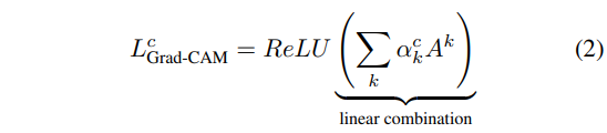
To compute Grad-CAM we’ll use the original paper equations and Stepan Ulyanin’s implementation of them.
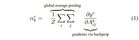
# pool the gradients across the channels
pooled_gradients = torch.mean(gradients[0], dim=[0, 2, 3])
import torch.nn.functional as F
import matplotlib.pyplot as plt

# weight the channels by corresponding gradients
for i in range(activations.size()[1]):
    activations[:, i, :, :] *= pooled_gradients[i]

# average the channels of the activations
heatmap = torch.mean(activations, dim=1).squeeze()

# relu on top of the heatmap
heatmap = F.relu(heatmap)

# normalize the heatmap
heatmap /= torch.max(heatmap)

# draw the heatmap
plt.matshow(heatmap.detach())
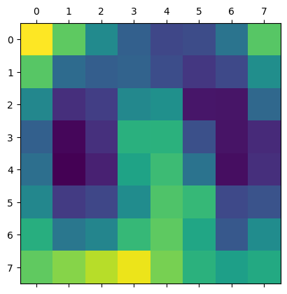
It’s worth noting that the activations we obtained through the forward hook contain 1,024 feature maps each capturing different aspects of the input image, each with a spatial resolution of 8x8.
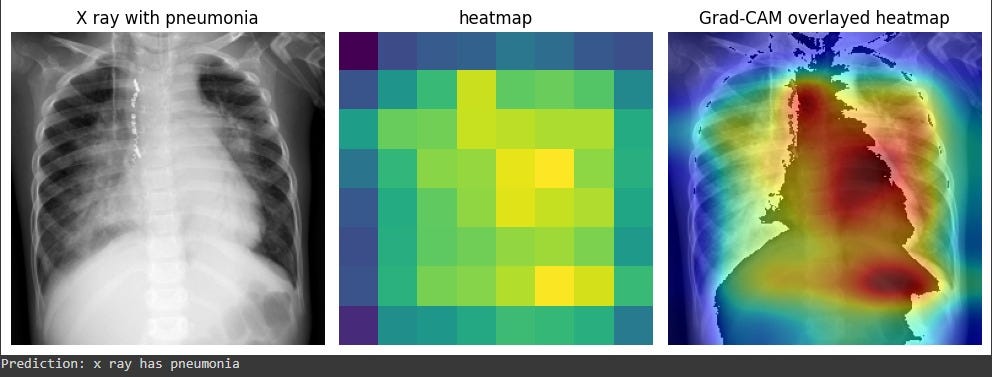
On the other hand, the gradients we obtained through the backward hook represent the importance of each feature map for the final prediction. By computing the element-wise product of the gradients and activations, we obtain a weighted sum of the feature maps, which highlights the most relevant parts of the image.
Finally, by computing the global average of the weighted feature maps, we obtain a single heatmap that indicates the regions of the image that are most important for the model’s prediction. This technique, known as Grad-CAM, provides a visual explanation of the model’s decision-making process and can help us interpret and debug the model’s behavior.
6. Combining the original image and the heatmap
The following code superimposes one image over another.
from torchvision.transforms.functional import to_pil_image
from matplotlib import colormaps
import numpy as np
import PIL

# Create a figure and plot the first image
fig, ax = plt.subplots()
ax.axis('off') # removes the axis markers

# First plot the original image
ax.imshow(to_pil_image(img_tensor, mode='RGB'))

# Resize the heatmap to the same size as the input image and defines
# a resample algorithm for increasing image resolution
# we need heatmap.detach() because it can't be converted to numpy array while
# requiring gradients
overlay = to_pil_image(heatmap.detach(), mode='F')
                      .resize((256,256), resample=PIL.Image.BICUBIC)

# Apply any colormap you want
cmap = colormaps['jet']
overlay = (255 * cmap(np.asarray(overlay) ** 2)[:, :, :3]).astype(np.uint8)

# Plot the heatmap on the same axes,
# but with alpha < 1 (this defines the transparency of the heatmap)
ax.imshow(overlay, alpha=0.4, interpolation='nearest', extent=extent)

# Show the plot
plt.show()

Finally, to remove the hooks from your model, you just need to call the remove method in each of the handles.
backward_hook.remove()
forward_hook.remove()
Conclusion
I hope this article helped clarify how Grad-CAM works, how to implement it using Pytorch, and how one can do it by using forward and backward hooks without changing the original model’s forward function.
I’d like to thank Stepan Ulyanin for his article and for helping me better understand Grad-CAM. I hope I could contribute something to readers as well.
I’d also like to leave the Python library torch-cam as a reference. It has other implementations of Grad-CAM, so you don’t need to do this from scratch.
Grad-CAM in Pytorch: Use of Forward and Backward Hooks was originally published in Towards Data Science on Medium, where people are continuing the conversation by highlighting and responding to this story.
from Towards Data Science - Medium
https://towardsdatascience.com/grad-cam-in-pytorch-use-of-forward-and-backward-hooks-7eba5e38d569?source=rss----7f60cf5620c9---4
via RiYo Analytics


No comments