https://ift.tt/xha439P An end-to-end open-source project using the latest MONAI Generative Models to produce chest X-ray images from radiol...
An end-to-end open-source project using the latest MONAI Generative Models to produce chest X-ray images from radiological reports text
Hi everybody! In this post, we will create a Latent Diffusion Model to generate Chest X-Ray images using the new open-source extension for MONAI, MONAI Generative Models!
Introduction
Generative AI has a huge potential for healthcare since it allows us to create models that learn the underlying patterns and structure of the training dataset. This way, we can use these generative models to create an unlimited amount of synthetic data with the same details and characteristics of real data but without their restrictions. Given its importance, we created MONAI Generative Models, an open-source extension to the MONAI platform containing the latest models (like Diffusion Models, Autoregressive Transformers, and Generative Adversarial Networks) and components that help with the training and evaluate generative models.

In this post, we will go through a complete project to create a Latent Diffusion Model (the same type of model as Stable Diffusion) capable of generating Chest X-Rays (CXR) images from radiological reports. Here, we tried to make the code easy to understand and to be adapted to different environments, so, although it is not the most efficient one, I hope you enjoy it!
You can find the complete open-source project at this GitHub repository, where in this post we are referencing to the release v0.2.
Dataset
First, we start with the dataset. In this project, we are using the MIMIC Dataset. To access this dataset, it is necessary to create an account at the Physionet portal. We will use MIMIC-CXR-JPG (which contains the JPG files) and MIMIC-CXR (that includes the radiological reports). Both datasets are under the PhysioNet Credentialed Health Data License 1.5.0. After completing the free training course, you can freely download the dataset using the instruction at the bottom of the dataset page. Originally, the CXR images have about +1000x1000 pixels. So, this step can take a while.
Chest X-ray images are a crucial tool to provide valuable information about the structures and organs within the chest cavity, including the lungs, heart, and blood vessels, and after download, we should have more than 350k of them! These images are one of the three different projections: Posterior-Anterior (PA), Anterior-Posterior (AP), and Lateral (LAT). For this project, we are interested only in the PA projection, the most common one where we can visualise most of the features mentioned in the radiological reports (ending with 96,162 images). Regarding the reports, we have 85,882 files, each containing several text sections. Here we will use the Findings (mainly explaining the contents in the image) and Impressions (summarising the report’s contents, like a conclusion). To make our models and training process more manageable, we will resize the images to have 512 pixels on the smallest axis. The list of scripts to automatically perform these initial steps can be found in here.
Models
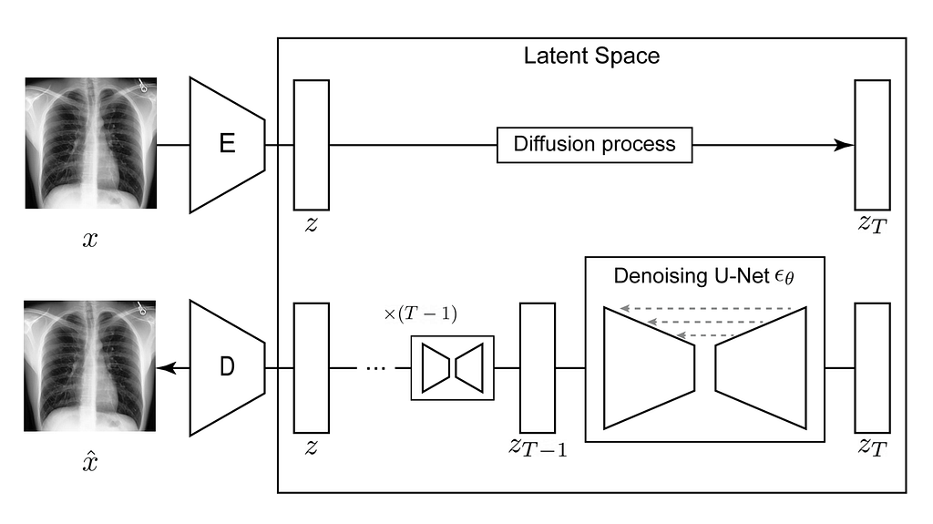
The Latent Diffusion Models are composed of several parts:
- An Autoencoder that performs the compression of the inputted images into a smaller latent representation;
- A Diffusion Model that will learn the probability data distribution of the latent representations of the CXR;
- A Text Encoder which creates an embedding vector that will condition the sampling process. In this example, we are using a pretrained one.
Using MONAI Generative Models, we can easily create and train these models, so let’s start with the Autoencoder!
Models — Autoencoder with KL regularization
The main goal of the Autoencoder with KL regularization (AE-kl or, in some projects, simply called as a VAE) is to be able to create a small latent representation, and also to reconstruct a image with high-fidelity (preserving as most as possible details). In this project, we are creating an autoencoder with four levels, with 64, 128, 128, 128 channels, where we apply a downsampling block between each level, making the feature maps smaller as we go to the deepest layers. Although our Autoencoder can have blocks with self-attention, in this example, we are adopting a structure similar to our previous study on brain images and using no attention to save memory usage. Finally, our latent representation has three channels.
from generative.networks.nets import AutoencoderKL

...

model = AutoencoderKL(
    spatial_dims=2,
    in_channels=1,
    out_channels=1,
    num_channels=[64, 128, 128, 128],
    latent_channels=3,
    num_res_blocks=2,
    attention_levels=[False, False, False, False],
    with_encoder_nonlocal_attn=False,
    with_decoder_nonlocal_attn=False,
)
Note: In our script, we are using the OmegaConf package to store the hyperparameters of our model. You can see the previous configuration in this file. In summary, OmegaConf is a powerful tool for managing configurations in Python projects, particularly those that involve deep learning or other complex software systems. OmegaConf allows us to conveniently organise the hyperparameters in the .yaml files and read them in the script.
Training AE-KL
Next, we define a few components of our training process. First, we have the KL regularisation. This part is responsible for evaluating the distance between the distribution of the latent space of the diffusion models and a Gaussian distribution. As proposed by Rombach et al., this will be used to restrict the variance of the latent space, which is useful when we train the diffusion model on it (more about it later). The forward method of our model returns the reconstruction, as well as the μ and σ vectors of our latent representation, which we use to compute the KL divergence.
# Inside training loop
reconstruction, z_mu, z_sigma = model(x=images)

…

kl_loss = 0.5 * torch.sum(z_mu.pow(2) + z_sigma.pow(2) - torch.log(z_sigma.pow(2)) - 1, dim=[1, 2, 3])
kl_loss = torch.sum(kl_loss) / kl_loss.shape[0]
Second, we have our Pixel-level loss, where in this project, we are adopting an L1 distance to evaluate how much our AE-kl reconstruction differs from the original image.
l1_loss = F.l1_loss(reconstruction.float(), images.float())
Next, we have our Perceptual-level loss. The idea of perceptual loss is that instead of evaluating the difference between the inputted image and the reconstruction at the pixel level, we pass both images through a pre-trained model. Then, we measure the distance of the internal activations and feature maps. In MONAI Generative models, we made it easy to use perceptual networks based on networks pre-trained on medical images (available here). We have access to the 2D networks from the RadImageNet study (from Mei et al.), which were trained on more than 1.3 million medical images! We implemented the 2.5D approach, using 2D pre-trained networks to evaluate 3D images by evaluating slices. And finally, we have access to MedicalNet to evaluate our 3D images in a 3D pure method. In this project, we are using a similar approach to Pinaya et al. and use the Learned Perceptual Image Patch Similarity (LPIPS) metric (also available at MONAI Generative Models).
# Instantiating the perceptual loss
perceptual_loss = PerceptualLoss(
     spatial_dims=2,
     network_type="squeeze",
)

...

# Inside training loop
...
p_loss = perceptual_loss(reconstruction.float(), images.float())
Finally, we use Adversarial loss to deal with the fine details of the reconstructions. The Adversarial Network was a Patch-Discriminator (initially proposed by the Pix2Pix study), where instead of having only one prediction about if the whole image was real or fake, we have predictions for several patches from the image.
Unlike the original Latent Diffusion Model and Stable Diffusion, we used discriminator losses from the least square GANs. Although it is not the more advanced adversarial loss, it has shown efficacy and stability when training on 3D medical images as well (but still room for improvement 😁). Although adversarial losses can be quite unstable, their combination with perceptual losses also helps to stabilise the loss of the discriminator and generator.
Our training loops and evaluation steps can be found at here and here. After train for 75 epoch, we save our model with the MLflow package. We use the MLflow package to better monitoring of our experiments since it organises information like git hash and parameters, as well as makes it possible to store different runs with a unique ID in groups (called experiments) and making easier to compare different results (similar to others tools, like weights and biases). The logs files for the AE-KL can be found here.
Models — Diffusion Model
Next, we need to train our diffusion model.
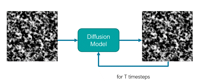
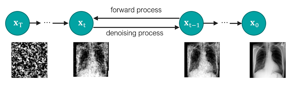
The diffusion model is a U-Net like network where traditionally, it receives a noisy image (or latent representation) as input and will predict its noise component. These models use an iterative denoising mechanism to generate images from noise across a Markov Chain with several steps. For this reason, the model is also conditioned on the timestep defining in which stage of the sampling process the model is.
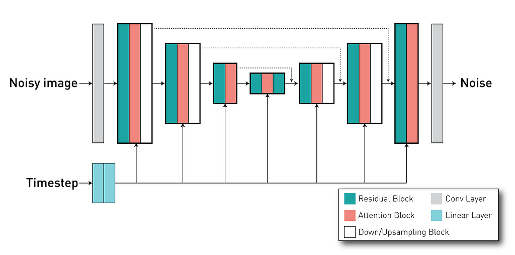
Using the DiffusionModelUNet class, we can create the U-Net like network for our diffusion mdel. Our project uses the configuration defined in this config file where it defines input and output with 3 channels (as our AE-kl have a latent space with 3 channels), and 3 different levels with 256, 512, 768 channels. Each level has 2 residual blocks. As mentioned, it is important to pass the timestep for the model where it is used to condition the behaviour of these residual blocks. Finally, we define the attention mechanisms inside the network. In our case, we have attention blocks in the second and third levels (indicated by the attention_levels argument), each with 512 and 768 channels per attention head (in other words, we have a single attention head in each level). These attention mechanisms are important because they allow us to apply our external conditioning (the radiological reports) to the network via the cross-attention method.
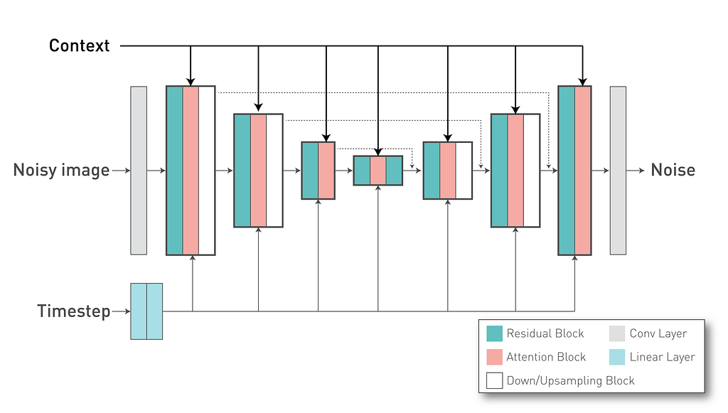
In our project, we are using an already trained textual encoder. For simplicity, we are using the same one from the Stable Diffusion v2.1 model (“stabilityai/stable-diffusion-2–1-base”) to convert our text tokens into a text embedding that will be used as Key and Value vectors in the DiffusionModel UNet cross attention layers. Each token of our textual embedding have 1024 dimensions and we define it in the “with_conditioning” and “cross_attention_dim” arguments.
from generative.networks.nets import DiffusionModelUNet

...

diffusion = DiffusionModelUNet(
    spatial_dims=2,
    in_channels=3,
    out_channels=3,
    num_res_blocks=2,
    num_channels=[256, 512, 768],
    attention_levels=[False, True, True],
    with_conditioning=True,
    cross_attention_dim=1024,
    num_head_channels=[0, 512, 768],
)
Besides our model definition, it is important to define how the noise of the diffusion model will be added to the inputted images during training and removed during the sampling. For that, we implemented the Schedulers classes to our MONAI Generative Models to define the noise schedulers. In this example, we will use a DDPMScheduler, with 1000 time steps and the following hyperparameters.
from generative.networks.schedulers import DDPMScheduler

...

scheduler = DDPMScheduler(
    beta_schedule="scaled_linear",
    num_train_timesteps=1000,
    beta_start=0.0015,
    beta_end=0.0205,
    prediction_type="v_prediction",
)
Here, we opted for a “v-prediction” approach, where our U-Net will try to predict the velocity component (a combination of the original image and the added noise) instead of just the added noise. This approach has been shown to have more stable training and faster convergence (also used in https://arxiv.org/abs/2210.02303).
Training Diffusion Model
Before training the Diffusion Model, we need to find an appropriate scaling factor. As mentioned in Rombach et al., the signal-to-noise ratio can affect the results obtained with the LDM, if the standard deviation of the latent space distribution is too high. If the values of the latent representation are too high, the maximum amount of Gaussian noise we add to it might not be enough to destroy all information. This way, during training, information of the original latent representation might be present when it was not supposed to be, making it not possible later sample an image from pure noise. The KL regularisation can help a little bit with this, but it is best practice to use a scaling factor to adapt the latent representation values. In this script, we verify the size of the standard deviation of the components of the latent space in one of the batches of the training set. We found that our scaling factor should be at least 0.8221. In our case, we used a more conservative value of 0.3 (similar to values from Stable Diffusion).
With the scaling factor defined, we can train our model. In here, we can check the training loop.
# Inside training loop
...

with torch.no_grad():
    e = stage1(images) * scale_factor
    prompt_embeds = text_encoder(reports.squeeze(1))[0]

timesteps = torch.randint(0, scheduler.num_train_timesteps, (images.shape[0],), device=device).long()
noise = torch.randn_like(e).to(device)
noisy_e = scheduler.add_noise(original_samples=e, noise=noise, timesteps=timesteps)
noise_pred = model(x=noisy_e, timesteps=timesteps, context=prompt_embeds)

if scheduler.prediction_type == "v_prediction":
    # Use v-prediction parameterization
    target = scheduler.get_velocity(e, noise, timesteps)
elif scheduler.prediction_type == "epsilon":
    target = noise

loss = F.mse_loss(noise_pred.float(), target.float())
As you can see, we first obtain the images and reports from our data loaders. To process our images, we used the transforms from MONAI and added a few custom transforms to extract random sentences from the radiological reports and tokenize the inputted text. In about 10% of the cases, we use an empty string (“” — which is a vector with the Begin-of-Sentence token (value = 49406) followed by padding tokens (value = 49407)) to be able to use classifier free guidance during the sampling.
Next, we obtain the latent representation and the prompt embeddings. We create the noise to be added, the random timesteps to be used in this iteration, and the desired target (velocity component). Finally, we compute our loss using the mean squared error.
This training goes for 500 epochs, where the logs can be found here.
Sampling images
After we have both models trained, we can sample synthetic images. We use this script.
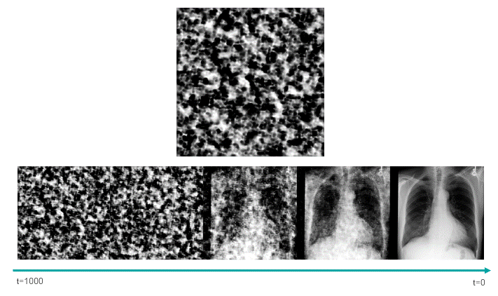
This script uses the classifier-free guidance, which is a method proposed by Ho et al., to be able to enforce the text prompts used in image generation. In this method, we have a guidance scale that we can use to sacrifice the diversity of the generated data to obtain a sample with higher fidelity to the textual prompt. 7.0 is the default value.
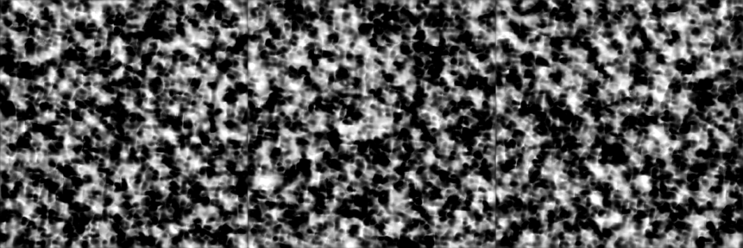
In the following image, we can see how the trained model was able to learn about the clinical features, as well as the position and severity of them.

Evaluation
In this section, we will show how to use metrics from MONAI to evaluate the performance of our generative models in several aspects.
Quality of the Autoencoder reconstructions with MS-SSIM
First, we verify how well our Autoencoder-kl reconstructs the input images. This is an important point when developing our models, because the quality of the compression and reconstructed data will define a ceiling for the quality of our sample. If the model does not learn how to decode the images from the latent representation well, or if it does not model our latent space well, it is not possible to decode the synthetic representations in a realistic way. In this script, we use the 5000 images from the test set to evaluate our model. We can verify how well our reconstructions look using the Multiscale Structural Similarity Index Measure (MS-SSIM). The MS-SSIM is a widely used image quality assessment method that measures the similarity between two images. Unlike traditional image quality assessment methods such as PSNR and SSIM, MS-SSIM is capable of capturing the structural information of an image at different scales.
In this case, the higher the value, the better the model. For our current release (version 0.2), we observed that our model had mean MS-SSIM reconstructions of 0.9789.
Diversity of the samples with MS-SSIM
We will first evaluate the diversity of the samples generated by our model. For that, we compute the Multiscale Structural Similarity Index Measure between different generated images. In this project, we assume that, if our generative model is capable of generating diverse images, it will present a low average MS-SSIM value when comparing pairs of synthetic images. For example, if we had a problem like a mode collapse, our generated images would look similar, and the MS-SSIM values would be much lower than what we observe in a real dataset.
In our project, we are using unconditioned samples (samples generated with the “” (empty string) as a textual prompt) to maintain the natural proportion of the original dataset. As shown in this script, we select 1000 synthetic samples of our model and use the data loaders from MONAI to help to load all possible pairs of images. We use a nested loop to go through all possible pairs and ignore the cases where it is the same image selected in both data loader. Here we can observe an MS-SSIM of 0.4083. We can perform the same evaluation in real images from the test set as a reference value. Using this script, we obtain MS-SSIM=0.4046 for the test set, indicating that our model is generating images with a diversity similar to the one observed at the real data.
However, diversity does not mean the images look good or realistic. So we will check the image quality in the next step!
Synthetic Image Quality with FID
Finally, we measure the Fréchet inception distance (FID) metric of the generated samples (link). The FID is a metric that evaluates the distribution between two groups, showing how similar they are. For this, we need a pre-trained neural network from which we can extract features that we will use to compute the distance (similar to the perceptual loss). In this example, we opted to use neural networks available in the torchxrayvision package. We used a Dense121 network (“densenet121-res224-all”), and we chose this network to be close to what is used in the literature for CXR synthetic images. From this network, we obtain a feature vector with 1024 dimensions. As recommended in the original FID paper, it is important to use a similar amount of examples compared to the number of features. For this reason, we use 1000 unconditioned images and compare them to 1000 images from the test set. For FIDs, the lower the best, and here we obtained a reasonable FID=9.0237.
Conclusion
In this post, we present a way to develop a project with MONAI Generative Models, from downloading the data to evaluating the generative models and synthetic data. Although this project version could be more efficient and have better hyperparameters, we hope that it illustrates well the different features our extension offers. If you have any idea on how to improve our CXR model or if you would like to contribute to our package, please, just add comments on our issue sections at here or here.
Our trained model can be found at the MONAI Model Zoo together with our 3D Brain Generator and other models. Our Model Zoo makes it easier downloading the model weights and the code to perform inference.
For more tutorials and to learn more about our features, check out our Tutorial page at this link, and follow me for the latest updates and more guides like this one! 😁
Note: All images unless otherwise noted are by the author
Generating Medical Images with MONAI was originally published in Towards Data Science on Medium, where people are continuing the conversation by highlighting and responding to this story.
from Towards Data Science - Medium
https://towardsdatascience.com/generating-medical-images-with-monai-e03310aa35e6?source=rss----7f60cf5620c9---4
via RiYo Analytics


ليست هناك تعليقات