Transformers in depth Part — 1 Introduction to Transformer models in 5 minutes

https://ift.tt/nTNMaUb Transformers in depth Part — 1 Introduction to Transformer models in 5 minutes Understanding Transformer architectu...

https://ift.tt/nTNMaUb

Transformers in depth Part — 1 Introduction to Transformer models in 5 minutes

Understanding Transformer architecture and its key insights in 5 minutes

This is the first part of the article’s extended version, soon you will find its continuation here.

Author’s note. For this very first part, I’ve decided to introduce the notions and concepts necessary to get a better understanding of Transformer models and to make it easier to follow the next chapter. If you are already familiar with Transformers, you can check the last section to get a summary of this article and feel free to jump to the second part, where more mathematics and complex notions are presented. Nevertheless, I hope you find some value in the explanations of this text too. Thanks for reading!

Since the release of the latest Large Language Models (LLaM), like the GPT series of OpenAI, the open source model Bloom or Google’s announcements about LaMDA among others, Transformers have demonstrated their huge potential and have become the cutting-edge architecture for Deep Learning models.

Although several articles have been written on transformers and the mathematics under their hood [2] [3] [4], in this series of articles I’d like to present a complete overview combining what I’ve considered the best approaches, with my own point of view and personal experience working with Transformer models.

This article attempts to provide a deep mathematical overview of Transformer models, showing the source of their power and explaining the reason behind each of its modules.

Note. The article follows the original transformer model from the paper Vaswani, Ashish, et al. 2017.

Setting the environment. A brief introduction to Natural Language Processing (NLP)

Before getting started with the Transformer model, it is necessary to understand the task for which they have been created, to process text.

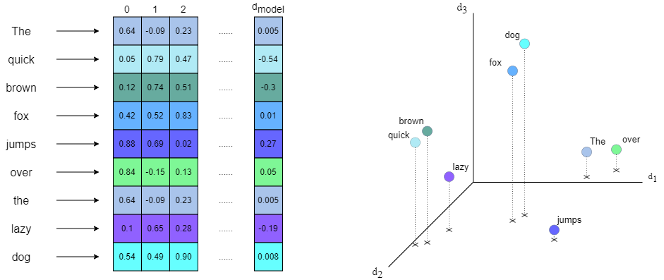
Since neural networks work with numbers, in order to feed text to a neural network we must first transform it into a numerical representation. The act of transforming text (or any other object) into a numerical form is called embedding. Ideally, the embedded representation is able to reproduce characteristics of the text such as the relationships between words or the sentiments of the text.
There are several ways to perform the embedding and it is not the purpose of this article to explain them (more information can be found in NLP Deep Learning), but rather we should understand their general mechanisms and the outputs they produce. If you are not familiar with embeddings, just think of them as another layer in the model’s architecture that transforms text into numbers.

The most commonly used embeddings work on the words of the text, transforming each word into a vector of a really high dimension (the elements into which the text is divided to apply the embedding are called tokens). In the original paper [1] the embedding dimension for each token/word was 512. It is important to note that the vector modulus is also normalized so the neural network is able to learn correctly and avoid exploding gradients.

An important element of embedding is the vocabulary. This corresponds to the set of all tokens (words) that can be used to feed the Transformer model. The vocabulary isn’t necessarily to be just the words used in the sentences, but rather any other word related to its topic. For instance, if the Transformer will be used to analyze legal documents, every word related to the bureaucratic jargon must be included in the vocabulary. Note that the larger the vocabulary (if it is related to the Transformer task), the better the embedding will be able to find relationships between tokens.

Apart from the words, there are some other special tokens added to the vocabulary and the text sequence. These tokens mark special parts of the text like the beginning <START>, the end <END>, or padding <PAD> (the padding is added so that all sequences have the same length). The special tokens are also embedded as vectors.

In mathematics, the embedding space constitutes a normalized vector space in which each vector corresponds to a specific token. The basis of the vector space is determined by the relationships the embedding layer has been able to find among the tokens. For example, one dimension might correspond to the verbs that end in -ing, another one could be the adjectives with positive meaning, etc. Moreover, the angle between vectors determines the similarity between tokens, forming clusters of tokens that have a semantic relationship.

Text embedding illustration. On the left, words/tokens are embedded as vectors where d_model represents the maximum embedding dimensions. On the right, the first 3 dimensions have been represented. Although the example is exaggerated, note how similar words form groups (clusters) representing the similarity between them. Image by the author.

Note 1. Although only the task of text processing has been mentioned, Transformers are in fact designed to process any type of sequential data.

Transformer’s workflow

Transformer diagram. Image from the paper Vaswani, Ashish, et al. 2017.

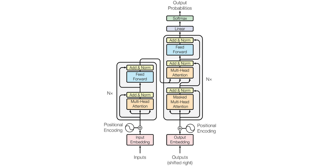
Above, is one of the most replicated diagrams in the last years of Deep Learning research. It summarizes the complete workflow of Transformers, representing each of the parts/modules involved in the process.

A higher perspective view divides Transformers into Encoder (left blue block in the diagram) and Decoder (right blue block).

To illustrate how Transformers work I will use the example task of text translation from Spanish to English.

Encoder’s objective is to find the relationships between the tokens of the input sequence i.e. the sentence to translate in Spanish. It gets the Spanish sentence as input (after applying the embedding) and outputs the same sequence weighted by the attention mechanism. Mathematically, the Encoder performs a transformation in the embedding space of Spanish tokens, weighting the vectors according to their importance in the sentence meaning.

Note 2. I haven’t defined yet what attention is, but essentially think of it as a function that returns some coefficients that define the importance of each word in the sentence with respect to the others.

On the other hand, Decoder takes as first input the translated sentence in English (Outputs in the original diagram), applies attention, and then combines the result with the encoder’s output in another attention mechanism. Intuitively, the Decoder learns to relate the target embedding space (English) with respect to the input embedding space (Spanish) so that it finds a basis transformation between both vector spaces.

Transformer’s high perspective overview. The Encoder and Decoder layers have been grouped into single blocks for simplicity, and the outputs of each block have been annotated. Image by the author.

Note 3. For clarity, I will use the notation source input to refer to the Encoder’s input (sentence in Spanish) and target input to the expected output introduced in the Decoder (sentence in English). This notation will remain consistent for the rest of the article.

Now let’s have a closer look at the Inputs (source and target) and the Output of the Transformer:

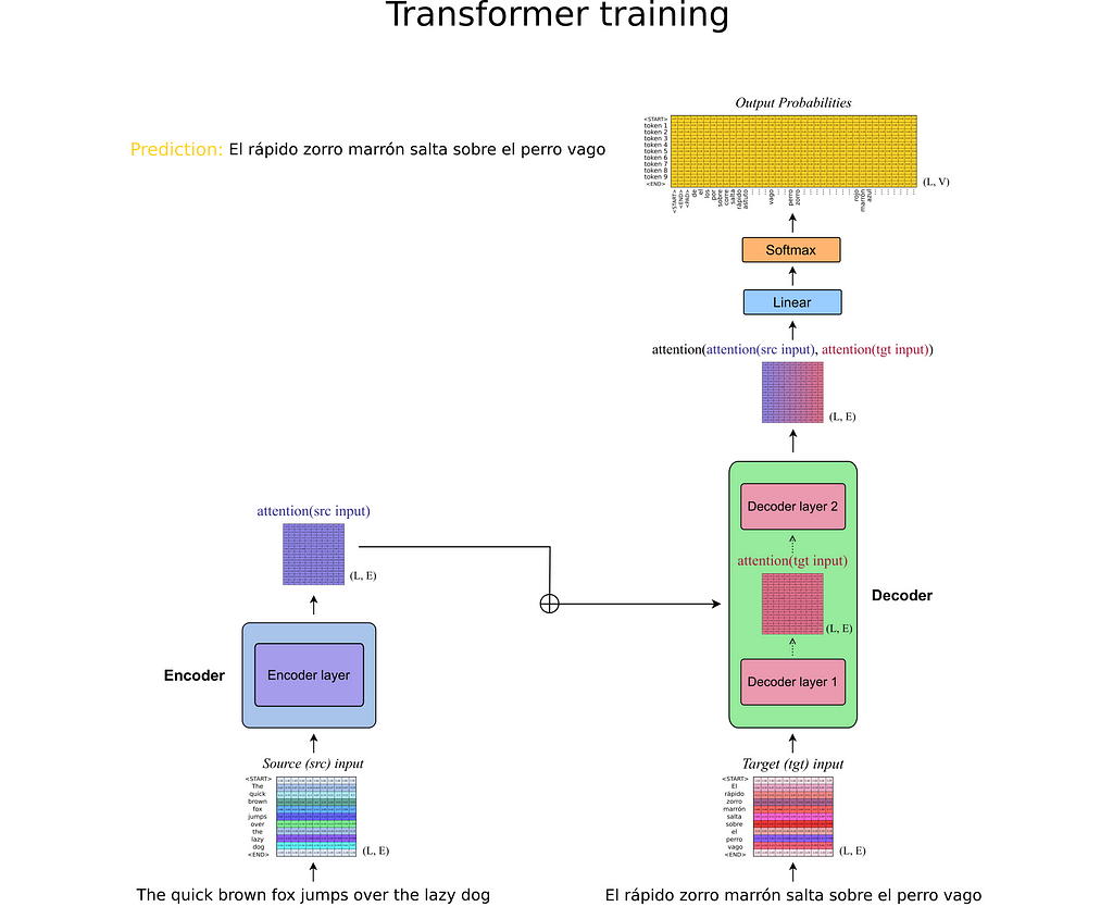
As we’ve seen, Transformer input text is embedded into a high dimensional vector space, so instead of a sentence, a sequence of vectors is entered. However, there exists a better mathematical structure to represent sequences of vectors, the matrices! And even further, when training a neural network, we don’t train it sample by sample, we rather use batches in which several samples are packed. The resulting input is a tensor of shape [N, L, E] where N is the batch size, L the sequence length, and E the embedding dimension.

Illustration of the **Source input tensor**. On the left, the 2D tensor representing the first **embedded sequence** of the batch. On the right, the full batch tensor containing all the sequences of a single batch that is fed into the Transformer Encoder. Similarly, the Target tensor has the same shape but contains the true output. Image by the author.

As for the output of the Transformer, a Linear + Softmax layer is applied which produces some Output Probabilities (recall that the Softmax layer outputs a probability distribution over the defined classes). The output of the Transformer isn’t the translated sentence but a probability distribution over the vocabulary that determines the words with the highest probability. Note that for each position in the sequence length, a probability distribution is generated to select the next token with a higher probability. Since during training the Transformer processes all the sentences at once, we get as output a 3D tensor that represents the probability distributions over the vocabulary tokens with shape [N, L, V] where N is the batch size, L the sequence length, and V the vocabulary length.

Illustration of the **Output Probabilities tensor**. On the left, the probability distribution prediction over the vocabulary for a single sequence. Each column represents a word in the vocabulary space, and the rows correspond to the sequence tokens. On the right, the full predicted tensor for a whole batch. Image by the author.

Finally, the predicted tokens are the ones with the highest probability.

Note 3. As explained in the Introduction to NLP section, all the sequences after the embedding have the same length, which corresponds to the longest possible sequence that can be introduced/produced in/by the Transformer.

Training vs Predicting

For the final section of the article’s Part 1, I’d like to make a point about the Training vs Predicting phases of Transformers.

As explained in the previous section, Transformers take two inputs (source and target). During Training, the Transformer is able to process all the inputs at once, meaning the input tensors are only passed one time through the model. The output is effectively the 3-dimensional probability tensor presented in the previous figure.

Transformer training phase. First, the source input (English sentence) is embedded and attention is applied in the Encoder. Then, the target input (Spanish) is entered into the Decoder, where source attention and target attention are combined in the Decider’s 2nd layer. Finally, the probability distribution over the vocabulary tokens is generated and the highest tokens are selected to form the translated output sentence. **Note that dimensions (L,E) do not change between layers**. Image by the author.

On the contrary, in the Prediction phase, there is no target input sequence to feed the Transformer (we wouldn’t need a Deep Learning model for text translation if we already know the translated sentence). So, what do we enter as target input?
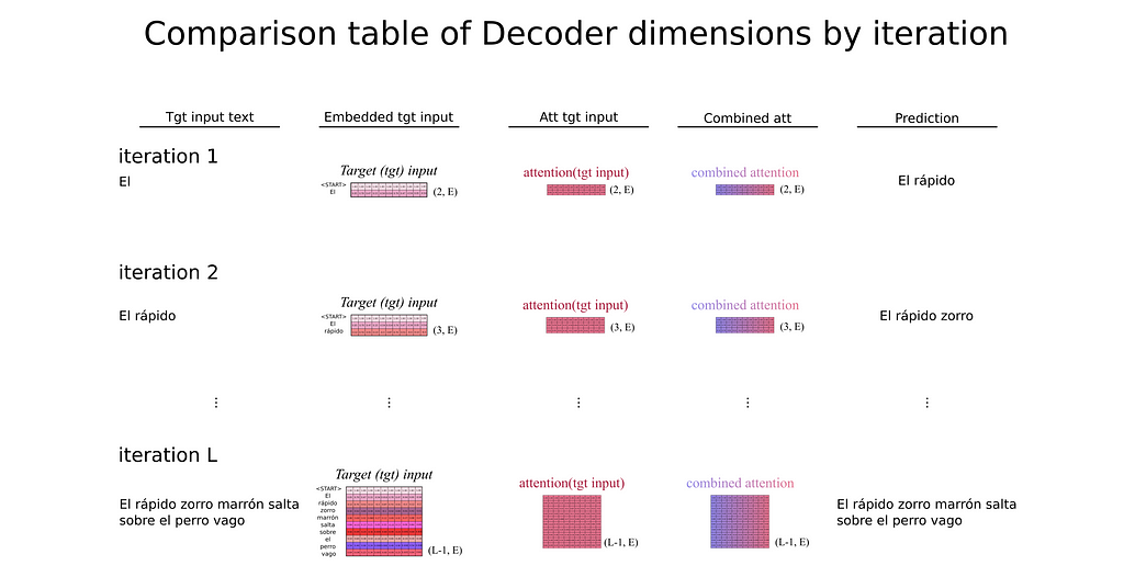
It is at this point that the auto-regressive behavior of Transformers comes to light. The Transformer can process the source input sequence at once in the Encoder, but for the Decoder’s module, it enters a loop where at each iteration it just produces the next token in the sequence (a row probability vector over the vocabulary tokens). The selected tokens with higher probability are then entered as the target input again so the Transformer always predicts the next token based on its previous predictions (hence the auto-regressive meaning). But what should be the first token entered at the very first iteration?
Remember the special tokens from the Introduction to NLP section? The first element introduced as target input is the beginning token <START> that marks the opening of the sentence.

Transformer predicting phase. The Encoder part remains unchanged, whereas Decoder’s tensors are row vectors. The input text for the first (0) iteration is empty since there is only the <START> token. **Note the arrow connecting the predicted token back to the target input representing the auto-regressive behavior**. In the next iterations, the target input will grow as the transformer predicts new tokens from the sequence. However, only the last row in the output probability tensor is taken into account, which means that the past predicted tokens cannot change. Image by the author.

Table comparing Decoder dimensions during predicting phase (iteration 0 is depicted in the above figure). Note the increase in dimensions from 1 to L-1. Once the Transformer has predicted the second last token in the sequence, it adds the <END> special token finishing the prediction. Image by the author.

Summary

This Part has been an Introduction to the first notions and concepts necessary to get a better understanding of Transformers models. In the next Part, I will delve into each of the modules of the Transformers architecture where most of the mathematics resides.

The main ideas and concepts behind this article are:

Transformers work in a normalized vector space defined by the embedding system and where each dimension represents a characteristic between tokens.
Transformers inputs are tensors of shape [N, L, E] where N denotes the batch size, L is the sequence length (constant for every sequence thanks to the padding) and E represents the embedding dimension.
While the Encoder finds relationships between tokens in the source embedding space, the Decoder’s task is to learn the projection from the source space into the target space.
Transformer’s output is a line vector whose length is equal to the vocabulary’s size and where each coefficient represents the probability of the corresponding indexed token being placed next in the sequence.
During training, Transformer processes all its inputs at once, outputting a [N, L, V] tensor (V is the vocabulary length). But during predicting, Transformers are auto-regressive, predicting token by token always based on their previous predictions.

Soon the next article’s part will be available here

Thanks for reading! If you’ve found this article helpful or inspiring, please consider following me for more content on AI and Deep Learning.

Gabriel Furnieles - Medium

Page Nav

Ads Place

Transformers in depth Part — 1 Introduction to Transformer models in 5 minutes

https://ift.tt/nTNMaUb Transformers in depth Part — 1 Introduction to Transformer models in 5 minutes Understanding Transformer architectu...