https://ift.tt/y9Bm86o SEIR Modeling in R Using deSolve — Chronic Wasting Disease in Deer Gaining health policy insight with small data se...
SEIR Modeling in R Using deSolve — Chronic Wasting Disease in Deer
Gaining health policy insight with small data sets
Collecting large amounts of data is a prerequisite for training and testing supervised machine learning models and making predictions. However, using small amounts of data and simple, yet foundational, mathematical models in R, we can generate large insights that can inform policy to alleviate infectious disease threats. These types of models are often overlooked in the data science community but are an equally important tool for generating insight.
One of the most prominent diseases ravaging deer and elk populations today is call Chronic Wasting Disease (CWD). CWD is a “transmissible spongiform encephalopathies or prion disease”, similar to mad cow disease, that “affects deer, elk, reindeer, sika deer and moose” [1, 2]. The disease is found in free-range deer populations and can be spread through “direct contact via body fluids like feces, saliva, blood, or urine or indirect contact via environmental contamination of soil, food or water” [2]. Currently, it does not affect humans, but keeping CWD-infected animals out of the food supply chain is an important goal of health security. Modeling the spread of the disease is important to understanding how CWD incidence might increase in the future. With some of the simple modeling tools I described in my previous blog post, we can build an SEIR model in R of CWD using data collected on white tail deer populations in Wisconsin.
SEIR Model
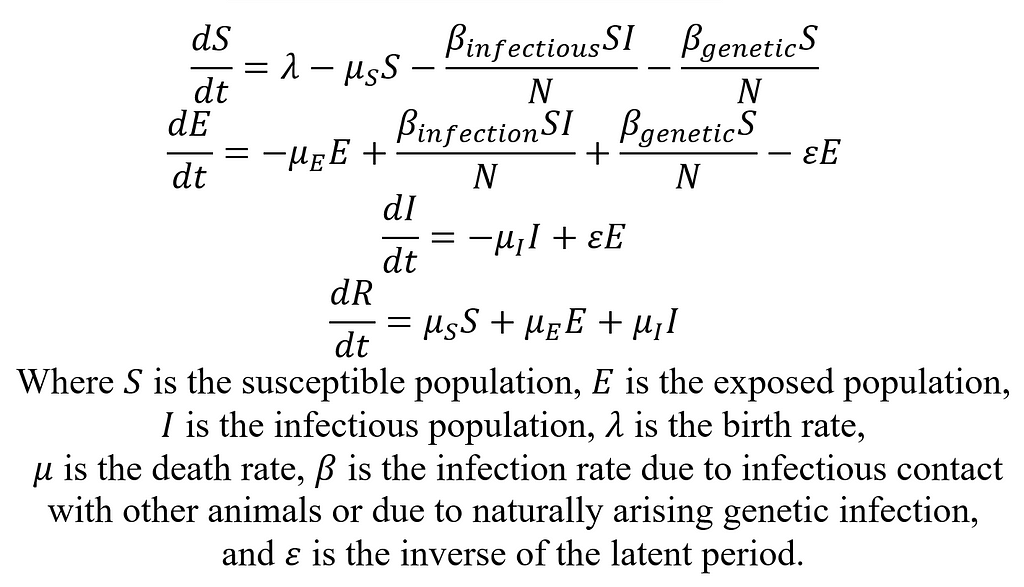
First, we will develop the simple SEIR model for CWD in a deer population. SEIR stands for Susceptible Exposed Infectious Recovered/Removed, and these disease states will form the basis for our compartmental model. In general, the susceptible state will include all deer not yet infected with CWD but who could be infected. There will be movement in and out of the susceptible state via births into the model, deaths out of the model, and infections. The exposed state of the model will include the population of deer that are infected with CWD but not yet infectious. Deer enter this stage after exposure to CWD until the latent period (time between becoming infected and becoming infectious) has passed. The infectious state is absorbing. That is to say, the only way out is through death. Now, let’s describe the SEIR model mathematically:
Parameters
Many of the parameter values can be instantiated through literature review or assumption upon consultation with a subject matter expert. Ideally, we want to minimize the number of parameters we calibrate. Many different parameter sets can achieve near identical fits to the data, and no parameter set will fit perfectly.
Sometimes, we find data in literature which can be manipulated to fit the form of our model. For example, the life expectancy of a deer is about 4.5 years [3], CWD has a latent period of about 15 months [1], and CWD increases mortality rate by about 4.5 times that of a healthy deer [4]. In addition, the state of Wisconsin publishes data on hunting harvests [5], which will inform our death rate, and on the number of hunting days [9]. The data on incidence of CWD (from 1999–2019) we will use in the model comes directly from test results published by the state of Wisconsin and can be found here: Summary of CWD Statewide Surveillance [8]. In the period for which we have data, about 99% of reported CWD cases occurred in the Southern Farmland Zone of Wisconsin, so we will limit our model population to that zone.
R Programming
First thing we do is import our data and define our model using the deSolve library. Here, we define our model as a function. Notice that we explicitly account for both natural deaths and deaths due to hunting as well as genetic (beta_CWD_Natural) and infectious (beta_CWD_Deer) CWD.
require('deSolve')
require('ggplot2')

#Original Data
df_1999_2019_SouthernFarmland <- read.csv('./CWD Year 1999-2019 Southern Farmland Population Only.csv')

##################
# Section 1. Model
##################
CWD_mod <- function(Time, State, Pars)
{
  with(as.list(c(State,Pars)),{
    N_Deer <- S_Deer + E_Deer + I_Deer
    births_in <- death_rate_S*S_Deer + hunt_kill_rate*S_Deer*N_Hunters + death_rate_E*E_Deer + hunt_kill_rate*E_Deer*N_Hunters + death_rate_I*I_Deer + hunt_kill_rate*I_Deer*N_Hunters
    d_S_Deer <- births_in - death_rate_S*S_Deer - beta_CWD_Deer*S_Deer*(I_Deer)/N_Deer - beta_CWD_Natural*S_Deer/N_Deer - hunt_kill_rate*S_Deer*N_Hunters
    d_E_Deer <- beta_CWD_Deer*S_Deer*(I_Deer)/N_Deer + beta_CWD_Natural*S_Deer/N_Deer - epsilon_Deer*E_Deer - death_rate_E*E_Deer - hunt_kill_rate*E_Deer*N_Hunters
    d_I_Deer <- epsilon_Deer*E_Deer - death_rate_I*I_Deer - hunt_kill_rate*I_Deer*N_Hunters
    return(list(c(d_S_Deer, d_E_Deer, d_I_Deer)))
  })
}
Now, we use a literature review and some informed assumptions to define all our parameters except for the transmission rate of CWD. For convenience, I included in the comments the websites/references I used to parameterize the model.
##########################
# Section 2. Parameters
##########################
S_Deer <- 1377100/4
E_Deer <- 0
I_Deer <- 3
births_in <- 100
life_expectancy_deer <- 4.5 # years https://www.jstor.org/stable/3803059?seq=7#metadata_info_tab_contents
life_expectancy_deer <- life_expectancy_deer * 12
death_rate_S <- 1/life_expectancy_deer
epsilon_Deer <- 1/15 #https://pdfs.semanticscholar.org/75eb/8b27d8cd507c23f2a74bfc7f4391505a7b4a.pdf
death_rate_E <- 1/(life_expectancy_deer)
risk_ratio_CWD_Deer <- 4.5 # https://www.dec.ny.gov/docs/wildlife_pdf/cwdfactsheet.pdf
death_rate_I <- death_rate_S * risk_ratio_CWD_Deer

hunter_harvest_2017 <- 322054 #https://dnr.wi.gov/wideermetrics/DeerStats.aspx
Avg_days_hunted_2017 <- 4.3 # https://dnr.wi.gov/topic/WildlifeHabitat/documents/reports/gundeer2.pdf
hunter_days_2017 <- 2695768 # https://dnr.wi.gov/topic/WildlifeHabitat/documents/reports/gundeer2.pdf
num_hunters_2017 <- 2695768/4.3
num_deer_2017 <- 1377100
num_deers_per_hunter_2017 <- hunter_harvest_2017/num_hunters_2017
hunter_kill_rate_year <- num_deers_per_hunter_2017/num_deer_2017
hunter_kill_rate_month <- hunter_kill_rate_year/12
beta_CWD_Natural <- .000001
Now, we have reached the all-important calibration step. As I mentioned before, there are many different parameter sets that will generate a good-fitting model. Our job now is to estimate the transmission rate of CWD that best fits the incidence data from Wisconsin given that we will hold all other parameters constant.
There are many different ways to calibrate a model, as parameter values have an infinite range of possibilities. For the transmission rate of CWD, the possible value of the transmission rate of CWD can range from 0 to positive infinity. In this case, I did some initial exploration that led me to believe the value of beta_CWD_Deer would be somewhere between 0.01 and 0.5. In this case, I will test all values between 0.01 and 0.5 in increments of 0.001. This is the simplest approach one could take, but when our focus is policy or simplicity, it will do just fine. We will look for the value of beta_CWD_Deer which will minimize the mean squared error between the number of cases recorded each year in the data and the number of cases reported each year by the model.
##########################
# Section 3. Calibration
##########################
beta_CWD_Deer <- 0.01

# Define list of possible values for beta_CWD_Deer
list_beta_CWD_Deer <- seq(0.01,0.5,by = 0.001)
# This is a placeholder value that also serves as a sanity check
best_beta_CWD_Deer <- 100
# Set the best score to something absurdly high as a santiy check
best_beta_CWD_Deer_Score <- 10000000000000000000000000

#Track for plot
list_all_betas <- c()
list_all_mse_scores <- c()

for(i in 1:length(list_beta_CWD_Deer))
{
  # Test the possible value of beta_CWD_Deer
  beta_CWD_Deer <- list_beta_CWD_Deer[i]
  #Initialize the model population
  ini_cwd_mod <- c(S_Deer = S_Deer, E_Deer = E_Deer, I_Deer = I_Deer)
  #Run the model for 252 months
  times_cwd_mod <- seq(1,252,by = 1) #By Month
  #Initialize the parameters in the model
  pars_cwd_mod <- c(births_in = births_in, death_rate_S = death_rate_S,
                    beta_CWD_Deer = beta_CWD_Deer,
                    beta_CWD_Natural = beta_CWD_Natural,
                    hunt_kill_rate = hunter_kill_rate_month,
                    epsilon_Deer = epsilon_Deer,
                    death_rate_E = death_rate_E,
                    death_rate_I = death_rate_I,
                    N_Hunters = num_hunters_2017)

  #Output using our previously defined function
  CWD_mod_Out <- ode(ini_cwd_mod, times_cwd_mod, CWD_mod, pars_cwd_mod)

  #create a data frame of the results
  yS_Deer <- CWD_mod_Out[,"S_Deer"]
  yE_Deer <- CWD_mod_Out[,"E_Deer"]
  yI_Deer <- CWD_mod_Out[,"I_Deer"]
  CWD_Results <- data.frame(yS_Deer, yE_Deer, yI_Deer)
  #Calculate the model predicted prevalence each year
  CWD_Results$Prevalence <- CWD_Results$yI_Deer / (CWD_Results$yS_Deer +
                                                     CWD_Results$yE_Deer +
                                                     CWD_Results$yI_Deer)
  CWD_Results_Year <- CWD_Results[c(12,24,36,48,60,72,84,96,108,120,
                                    132,144,156,168,180,192,204,
                                    216,228,240,252),]
  # Compare to the data
  CWD_Results_Year$Prevalence_Data <- df_1999_2019_SouthernFarmland$Incidence
  CWD_Results_Year$Year <- df_1999_2019_SouthernFarmland$Year

  CWD_Results_Year$Prevalence_Data <- as.numeric(as.character(CWD_Results_Year$Prevalence_Data))
  CWD_Results_Year$Prevalence <- as.numeric(as.character(CWD_Results_Year$Prevalence))
  # Calculate the mean squared error
  curr_mean_sq_err <- mean((CWD_Results_Year$Prevalence - CWD_Results_Year$Prevalence_Data)^2)

  list_all_betas <- c(list_all_betas, beta_CWD_Deer)
  list_all_mse_scores <- c(list_all_mse_scores, curr_mean_sq_err)

  #If it is the lowest MSE, save the beta value and the score as the best
  if(curr_mean_sq_err < best_beta_CWD_Deer_Score)
  {
    best_beta_CWD_Deer <- beta_CWD_Deer
    best_beta_CWD_Deer_Score <- curr_mean_sq_err
    print(curr_mean_sq_err)
  }
  print(i)
}
We can plot the mean squared error over time using ggplot to visually see how the model improves with different parameter values.
plot_df <- as.data.frame(matrix(c(list_all_betas, list_all_mse_scores), ncol = 2, byrow = FALSE))
colnames(plot_df) <- c('beta_CWD_Deer', 'Model_MSE')

ggplot()+
  geom_line(data = plot_df, aes(x = beta_CWD_Deer, y = Model_MSE, color = 'Model MSE'), size = 3)+
  xlab('beta_CWD_Deer Value')+
  ylab('MSE')+
  ggtitle('Calibration Results')+
  theme_bw()+
  theme(axis.text.x = element_text(size = 24),
        axis.text.y = element_text(size = 24),
        axis.title = element_text(size = 28),
        axis.title.x = element_text(size = 28),
        axis.title.y = element_text(size = 28),
        title = element_text(size = 16),
        legend.text = element_text(size = 24))+
  scale_color_brewer(palette="Pastel1")+
  theme(panel.grid.major = element_blank(), panel.grid.minor = element_blank())+
  labs(color=' ', shape = '')
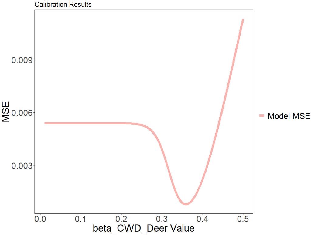
The value of beta_CWD_Deer which minimizes model error is 0.359. We can see from the graph that, with a value below around 0.25, the outbreak never occurs and, therefore, the error is constant.
Results
Now, we can run our full model with the assumed and calibrated parameter set.
###############################################
# Section 4. Plot Results
###############################################

beta_CWD_Deer <- best_beta_CWD_Deer

ini_cwd_mod <- c(S_Deer = S_Deer, E_Deer = E_Deer, I_Deer = I_Deer)

times_cwd_mod <- seq(1,252,by = 1) #By Month

pars_cwd_mod <- c(births_in = births_in, death_rate_S = death_rate_S,
                  beta_CWD_Deer = beta_CWD_Deer,
                  beta_CWD_Natural = beta_CWD_Natural,
                  hunt_kill_rate = hunter_kill_rate_month,
                  epsilon_Deer = epsilon_Deer,
                  death_rate_E = death_rate_E,
                  death_rate_I = death_rate_I,
                  N_Hunters = num_hunters_2017)

#Output
CWD_mod_Out <- ode(ini_cwd_mod, times_cwd_mod, CWD_mod, pars_cwd_mod)

yS_Deer <- CWD_mod_Out[,"S_Deer"]
yE_Deer <- CWD_mod_Out[,"E_Deer"]
yI_Deer <- CWD_mod_Out[,"I_Deer"]
CWD_Results <- data.frame(yS_Deer, yE_Deer, yI_Deer)
CWD_Results$Prevalence <- CWD_Results$yI_Deer / (CWD_Results$yS_Deer +
                                                  CWD_Results$yE_Deer +
                                                  CWD_Results$yI_Deer)
CWD_Results_Year <- CWD_Results[c(12,24,36,48,60,72,84,96,108,120,
                                  132,144,156,168,180,192,204,
                                  216,228,240,252),]
CWD_Results_Year$Prevalence_Data <- df_1999_2019_SouthernFarmland$Incidence
CWD_Results_Year$Year <- df_1999_2019_SouthernFarmland$Year

CWD_Results$Year <- seq((1998+(1/12)),2019,by=(1/12))

ggplot()+
  geom_point(data = df_1999_2019_SouthernFarmland, aes(x = Year, y = Incidence, color = 'Southern Farmland Zone Data'), size = 3)+
  geom_line(data = CWD_Results, aes(x = Year, y = Prevalence, color = 'Model'), size = 2)+
  xlab('Year')+
  ylab('Prevalence')+
  ggtitle('Chronic Wasting Disease, Whitetail Deer, Wisconsin')+
  theme_bw()+
  theme(axis.text.x = element_text(size = 24),
        axis.text.y = element_text(size = 24),
        axis.title = element_text(size = 28),
        axis.title.x = element_text(size = 28),
        axis.title.y = element_text(size = 28),
        title = element_text(size = 16),
        legend.text = element_text(size = 24),
        legend.position = c(0.3,0.9))+
  scale_y_continuous(breaks = c(0,0.05,0.1,0.15),
                     labels = c('0%','5%','10%','15%'))+
  scale_x_continuous(breaks = c(1999,2005,2011,2017),
                     labels = c('1999', '2005', '2011', '2017'))+
  scale_color_brewer(palette="Pastel1")+
  theme(panel.grid.major = element_blank(), panel.grid.minor = element_blank())+
  labs(color=' ', shape = '')
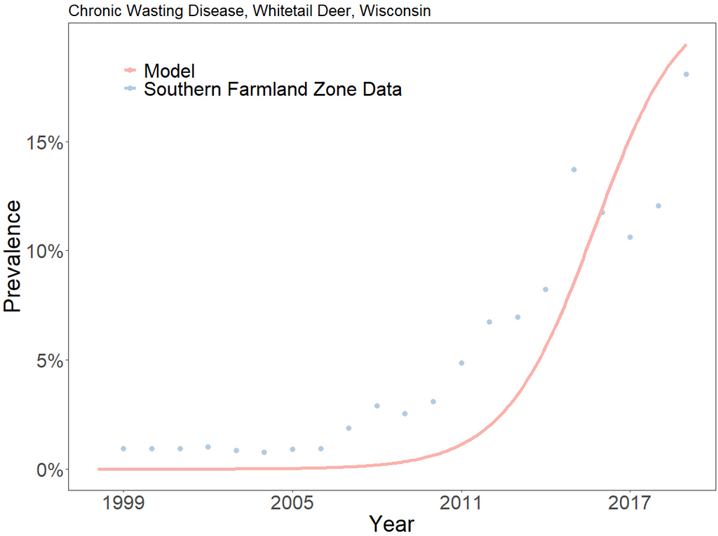
From the graph, we can see that the model underfits CWD prevalence until 2016. Then, the model begins to overfit prevalence. The SEIR model will never fit the data perfectly, nor is it designed to do so. It is meant to serve as an elegant approximation for disease spread. We can run the model beyond the period for which we have data to see what will happen in the long-term:
###############################################
# Section 5. Plot Predicted prevalence 10 years forward
###############################################

beta_CWD_Deer <- best_beta_CWD_Deer

ini_cwd_mod <- c(S_Deer = S_Deer, E_Deer = E_Deer, I_Deer = I_Deer)

times_cwd_mod <- seq(1,492,by = 1) #By Month

pars_cwd_mod <- c(births_in = births_in, death_rate_S = death_rate_S,
                  beta_CWD_Deer = beta_CWD_Deer,
                  beta_CWD_Natural = beta_CWD_Natural,
                  hunt_kill_rate = hunter_kill_rate_month,
                  epsilon_Deer = epsilon_Deer,
                  death_rate_E = death_rate_E,
                  death_rate_I = death_rate_I,
                  N_Hunters = num_hunters_2017)

#Output
CWD_mod_Out <- ode(ini_cwd_mod, times_cwd_mod, CWD_mod, pars_cwd_mod)

yS_Deer <- CWD_mod_Out[,"S_Deer"]
yE_Deer <- CWD_mod_Out[,"E_Deer"]
yI_Deer <- CWD_mod_Out[,"I_Deer"]
CWD_Results <- data.frame(yS_Deer, yE_Deer, yI_Deer)
CWD_Results$Prevalence <- CWD_Results$yI_Deer / (CWD_Results$yS_Deer +
                                                   CWD_Results$yE_Deer +
                                                   CWD_Results$yI_Deer)
CWD_Results_Year <- CWD_Results[c(12,24,36,48,60,72,84,96,108,120,
                                  132,144,156,168,180,192,204,
                                  216,228,240,252,
                                  264,276,288,300,
                                  312,324,336,348,360,372,
                                  384,396,408,420,432,
                                  444,456,468,480,492),]

CWD_Results$Year <- seq((1998+(1/12)),2039,by=(1/12))

ggplot()+
  geom_point(data = df_1999_2019_SouthernFarmland, aes(x = Year, y = Incidence, color = 'Southern Farmland Zone Data'), size = 3)+
  geom_line(data = CWD_Results, aes(x = Year, y = Prevalence, color = 'Model'), size = 2)+
  xlab('Year')+
  ylab('Prevalence')+
  ggtitle('Chronic Wasting Disease, Whitetail Deer, Wisconsin')+
  theme_bw()+
  theme(axis.text.x = element_text(size = 24),
        axis.text.y = element_text(size = 24),
        axis.title = element_text(size = 28),
        axis.title.x = element_text(size = 28),
        axis.title.y = element_text(size = 28),
        title = element_text(size = 16),
        legend.text = element_text(size = 24),
        legend.position = c(0.3,0.9))+
  scale_y_continuous(breaks = c(0,0.05,0.1,0.15),
                     labels = c('0%','5%','10%','15%'))+
  scale_x_continuous(breaks = c(2000,2005,2010,2015,2020,2025,2030,2035),
                     labels = c('2000','2005','2010','2015','2020','2025','2030','2035'))+
  scale_color_brewer(palette="Pastel1")+
  theme(panel.grid.major = element_blank(), panel.grid.minor = element_blank())+
  labs(color=' ', shape = '')
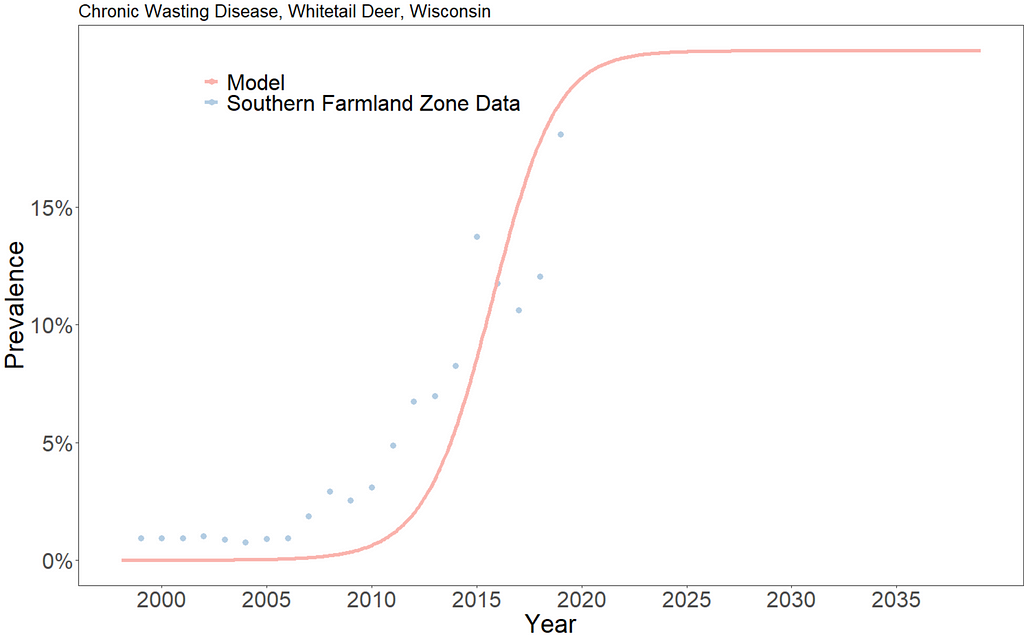
The model predicts a relatively steady 22% CWD prevalence in the population starting in 2023. This should be understood to mean that if the underlying disease and population dynamics do not change, the southern farmland region of Wisconsin should expect a CWD prevalence in white tail deer of about 22%.
In 2022, the Wisconsin Department of Natural Resources identified a prevalence of a little over 18% [6].
Policy Evaluation
Now that we have our model and baseline projections, we can explore some hypothetical interventions and their effects on CWD spread. For example, Current hunting regulations authorize the killing of one deer per permit in Wisconsin [7]. However, the state government is considering allowing unlimited kills of deer presenting symptoms of CWD. Let’s imagine several possible scenarios:
- The law is expected to increase the rate of hunting deer with CWD by 35% and without CWD by 15% (due to misdiagnoses).
- The law is enacted, but the prion disease has mutated to become 30% more contagious.
- The law is enacted, the prion disease mutated, and new AI-assisted technology was developed that uses computer vision to perfectly classify infected vs non-infected deer. Therefore, the law is expected to increase the rate of hunting deer with CWD by 70% and without CWD by 0%.
In the model, we will treat the scenarios as all beginning in 2020 (when we have no data). While we will be adjusting the hunting rate and transmission rate, we will continue to keep the simplifying assumption that the population stays constant (births in = deaths out). Here is the R code to implement and plot our scenario comparison:
###################################
# Section 6. Policy Evaluation
###################################

# Run period with data
beta_CWD_Deer <- best_beta_CWD_Deer

ini_cwd_mod <- c(S_Deer = S_Deer, E_Deer = E_Deer, I_Deer = I_Deer)

times_cwd_mod <- seq(1,252,by = 1) #By Month

pars_cwd_mod <- c(births_in = births_in, death_rate_S = death_rate_S,
                  beta_CWD_Deer = beta_CWD_Deer,
                  beta_CWD_Natural = beta_CWD_Natural,
                  hunt_kill_rate = hunter_kill_rate_month,
                  epsilon_Deer = epsilon_Deer,
                  death_rate_E = death_rate_E,
                  death_rate_I = death_rate_I,
                  N_Hunters = num_hunters_2017)

#Output
CWD_mod_Out <- ode(ini_cwd_mod, times_cwd_mod, CWD_mod, pars_cwd_mod)

yS_Deer <- CWD_mod_Out[,"S_Deer"]
yE_Deer <- CWD_mod_Out[,"E_Deer"]
yI_Deer <- CWD_mod_Out[,"I_Deer"]
CWD_Results_data <- data.frame(yS_Deer, yE_Deer, yI_Deer)
CWD_Results_data$Prevalence <- CWD_Results_data$yI_Deer / (CWD_Results_data$yS_Deer +
                                                             CWD_Results_data$yE_Deer +
                                                             CWD_Results_data$yI_Deer)
CWD_Results_data$Year <- seq((1998+(1/12)),2019,by=(1/12))

# Baseline model continues 20 years
beta_CWD_Deer <- best_beta_CWD_Deer

ini_cwd_mod <- c(S_Deer = CWD_Results_data$yS_Deer[252], E_Deer = CWD_Results_data$yE_Deer[252], I_Deer = CWD_Results_data$yI_Deer[252])

times_cwd_mod <- seq(253,492,by = 1) #By Month

pars_cwd_mod <- c(births_in = births_in, death_rate_S = death_rate_S,
                  beta_CWD_Deer = beta_CWD_Deer,
                  beta_CWD_Natural = beta_CWD_Natural,
                  hunt_kill_rate = hunter_kill_rate_month,
                  epsilon_Deer = epsilon_Deer,
                  death_rate_E = death_rate_E,
                  death_rate_I = death_rate_I,
                  N_Hunters = num_hunters_2017)

#Output
CWD_mod_Out <- ode(ini_cwd_mod, times_cwd_mod, CWD_mod, pars_cwd_mod)

yS_Deer <- CWD_mod_Out[,"S_Deer"]
yE_Deer <- CWD_mod_Out[,"E_Deer"]
yI_Deer <- CWD_mod_Out[,"I_Deer"]
CWD_Results_baseline_projection <- data.frame(yS_Deer, yE_Deer, yI_Deer)
CWD_Results_baseline_projection$Prevalence <- CWD_Results_baseline_projection$yI_Deer / (CWD_Results_baseline_projection$yS_Deer +
                                                                                           CWD_Results_baseline_projection$yE_Deer +
                                                                                           CWD_Results_baseline_projection$yI_Deer)
CWD_Results_baseline_projection$Year <- seq((2019+(1/12)),2039,by=(1/12))

# Scenario 1 model continues 20 years
CWD_mod_diff_hunt_rates <- function(Time, State, Pars)
{
  with(as.list(c(State,Pars)),{
    N_Deer <- S_Deer + E_Deer + I_Deer
    births_in <- death_rate_S*S_Deer + hunt_kill_rate_S*S_Deer*N_Hunters + death_rate_E*E_Deer + hunt_kill_rate_EI*E_Deer*N_Hunters + death_rate_I*I_Deer + hunt_kill_rate_EI*I_Deer*N_Hunters
    d_S_Deer <- births_in - death_rate_S*S_Deer - beta_CWD_Deer*S_Deer*(I_Deer)/N_Deer - beta_CWD_Natural*S_Deer/N_Deer - hunt_kill_rate_S*S_Deer*N_Hunters
    d_E_Deer <- beta_CWD_Deer*S_Deer*(I_Deer)/N_Deer + beta_CWD_Natural*S_Deer/N_Deer - epsilon_Deer*E_Deer - death_rate_E*E_Deer - hunt_kill_rate_EI*E_Deer*N_Hunters
    d_I_Deer <- epsilon_Deer*E_Deer - death_rate_I*I_Deer - hunt_kill_rate_EI*I_Deer*N_Hunters
    return(list(c(d_S_Deer, d_E_Deer, d_I_Deer)))
  })
}

beta_CWD_Deer <- best_beta_CWD_Deer

ini_cwd_mod <- c(S_Deer = CWD_Results_data$yS_Deer[252], E_Deer = CWD_Results_data$yE_Deer[252], I_Deer = CWD_Results_data$yI_Deer[252])

times_cwd_mod <- seq(253,492,by = 1) #By Month

pars_cwd_mod <- c(births_in = births_in, death_rate_S = death_rate_S,
                  beta_CWD_Deer = beta_CWD_Deer,
                  beta_CWD_Natural = beta_CWD_Natural,
                  hunt_kill_rate_S = hunter_kill_rate_month*1.15,
                  hunt_kill_rate_EI = hunter_kill_rate_month*1.35,
                  epsilon_Deer = epsilon_Deer,
                  death_rate_E = death_rate_E,
                  death_rate_I = death_rate_I,
                  N_Hunters = num_hunters_2017)

#Output
CWD_mod_Out <- ode(ini_cwd_mod, times_cwd_mod, CWD_mod_diff_hunt_rates, pars_cwd_mod)

yS_Deer <- CWD_mod_Out[,"S_Deer"]
yE_Deer <- CWD_mod_Out[,"E_Deer"]
yI_Deer <- CWD_mod_Out[,"I_Deer"]
CWD_Results_scenario_1_projection <- data.frame(yS_Deer, yE_Deer, yI_Deer)
CWD_Results_scenario_1_projection$Prevalence <- CWD_Results_scenario_1_projection$yI_Deer / (CWD_Results_scenario_1_projection$yS_Deer +
                                                                                               CWD_Results_scenario_1_projection$yE_Deer +
                                                                                               CWD_Results_scenario_1_projection$yI_Deer)
CWD_Results_scenario_1_projection$Year <- seq((2019+(1/12)),2039,by=(1/12))

# Scenario 2 model continues 20 years
beta_CWD_Deer <- best_beta_CWD_Deer*1.3

ini_cwd_mod <- c(S_Deer = CWD_Results_data$yS_Deer[252], E_Deer = CWD_Results_data$yE_Deer[252], I_Deer = CWD_Results_data$yI_Deer[252])

times_cwd_mod <- seq(253,492,by = 1) #By Month

pars_cwd_mod <- c(births_in = births_in, death_rate_S = death_rate_S,
                  beta_CWD_Deer = beta_CWD_Deer,
                  beta_CWD_Natural = beta_CWD_Natural,
                  hunt_kill_rate_S = hunter_kill_rate_month*1.15,
                  hunt_kill_rate_EI = hunter_kill_rate_month*1.35,
                  epsilon_Deer = epsilon_Deer,
                  death_rate_E = death_rate_E,
                  death_rate_I = death_rate_I,
                  N_Hunters = num_hunters_2017)

#Output
CWD_mod_Out <- ode(ini_cwd_mod, times_cwd_mod, CWD_mod_diff_hunt_rates, pars_cwd_mod)

yS_Deer <- CWD_mod_Out[,"S_Deer"]
yE_Deer <- CWD_mod_Out[,"E_Deer"]
yI_Deer <- CWD_mod_Out[,"I_Deer"]
CWD_Results_scenario_2_projection <- data.frame(yS_Deer, yE_Deer, yI_Deer)
CWD_Results_scenario_2_projection$Prevalence <- CWD_Results_scenario_2_projection$yI_Deer / (CWD_Results_scenario_2_projection$yS_Deer +
                                                                                               CWD_Results_scenario_2_projection$yE_Deer +
                                                                                               CWD_Results_scenario_2_projection$yI_Deer)
CWD_Results_scenario_2_projection$Year <- seq((2019+(1/12)),2039,by=(1/12))

# Scenario 3 model continues 20 years
beta_CWD_Deer <- best_beta_CWD_Deer*1.3

ini_cwd_mod <- c(S_Deer = CWD_Results_data$yS_Deer[252], E_Deer = CWD_Results_data$yE_Deer[252], I_Deer = CWD_Results_data$yI_Deer[252])

times_cwd_mod <- seq(253,492,by = 1) #By Month

pars_cwd_mod <- c(births_in = births_in, death_rate_S = death_rate_S,
                  beta_CWD_Deer = beta_CWD_Deer,
                  beta_CWD_Natural = beta_CWD_Natural,
                  hunt_kill_rate_S = hunter_kill_rate_month,
                  hunt_kill_rate_EI = hunter_kill_rate_month*1.7,
                  epsilon_Deer = epsilon_Deer,
                  death_rate_E = death_rate_E,
                  death_rate_I = death_rate_I,
                  N_Hunters = num_hunters_2017)

#Output
CWD_mod_Out <- ode(ini_cwd_mod, times_cwd_mod, CWD_mod_diff_hunt_rates, pars_cwd_mod)

yS_Deer <- CWD_mod_Out[,"S_Deer"]
yE_Deer <- CWD_mod_Out[,"E_Deer"]
yI_Deer <- CWD_mod_Out[,"I_Deer"]
CWD_Results_scenario_3_projection <- data.frame(yS_Deer, yE_Deer, yI_Deer)
CWD_Results_scenario_3_projection$Prevalence <- CWD_Results_scenario_3_projection$yI_Deer / (CWD_Results_scenario_3_projection$yS_Deer +
                                                                                               CWD_Results_scenario_3_projection$yE_Deer +
                                                                                               CWD_Results_scenario_3_projection$yI_Deer)
CWD_Results_scenario_3_projection$Year <- seq((2019+(1/12)),2039,by=(1/12))

ggplot()+
  geom_point(data = df_1999_2019_SouthernFarmland, aes(x = Year, y = Incidence, color = 'Southern Farmland Zone Data'), size = 3)+
  geom_line(data = CWD_Results_data, aes(x = Year, y = Prevalence, color = 'Calibrated Model'), size = 2)+
  geom_line(data = CWD_Results_baseline_projection, aes(x = Year, y = Prevalence, color = 'Baseline Projection'), size = 2)+
  geom_line(data = CWD_Results_scenario_1_projection, aes(x = Year, y = Prevalence, color = 'Scenario 1 Projection'), size = 2)+
  geom_line(data = CWD_Results_scenario_2_projection, aes(x = Year, y = Prevalence, color = 'Scenario 2 Projection'), size = 2)+
  geom_line(data = CWD_Results_scenario_3_projection, aes(x = Year, y = Prevalence, color = 'Scenario 3 Projection'), size = 2)+
  xlab('Year')+
  ylab('Prevalence')+
  ggtitle('Chronic Wasting Disease, Whitetail Deer, Wisconsin')+
  theme_bw()+
  theme(axis.text.x = element_text(size = 24),
        axis.text.y = element_text(size = 24),
        axis.title = element_text(size = 28),
        axis.title.x = element_text(size = 28),
        axis.title.y = element_text(size = 28),
        title = element_text(size = 16),
        legend.text = element_text(size = 24),
        legend.position = c(0.2,0.8))+
  scale_y_continuous(breaks = c(0,0.05,0.1,0.15),
                     labels = c('0%','5%','10%','15%'))+
  scale_x_continuous(breaks = c(2000,2005,2010,2015,2020,2025,2030,2035),
                     labels = c('2000','2005','2010','2015','2020','2025','2030','2035'))+
  theme(panel.grid.major = element_blank(), panel.grid.minor = element_blank())+
  labs(color=' ', shape = '')
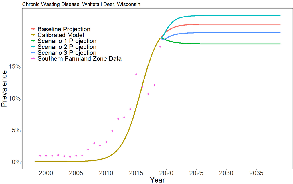
We can see that increasing hunting of CWD-infected deer has very little overall effect on the prevalence of CWD. Scenario 1 results in a long-term prevalence of about 18.5%, scenario 2 results in a long-term prevalence of about 23%, and scenario 3 results in a long-term prevalence of about 20.2%. In reality, there are additional environmental and ecological consequences that we do not consider in this approach.
Conclusions
With only 20 data points, we were able to develop a simple model that explains the spread of CWD in the whitetail deer population in southern Wisconsin using the SEIR model. Such models are especially useful at informing policy when combined with subject matter expertise. While not as accurate or as novel as AI methods, mathematical models perform astoundingly well with very small amounts of data.
All images unless otherwise noted are by the author.
Data was used under written permission of the Wisconsin Department of Natural Resources.
References
[1] Williams ES, Miller MW. Chronic wasting disease in deer and elk in North America. Rev Sci Tech. 2002 Aug;21(2):305–16. doi: 10.20506/rst.21.2.1340. PMID: 11974617.
[2] Centers for Disease Control and Prevention. Chronic Wasting Disease (CWD) | Prion Diseases | CDC. 2023.
[3] Lopez, R. R., Mark E. P. Vieira, Silvy, N. J., Frank, P. A., Whisenant, S. W., & Jones, D. A. (2003). Survival, Mortality, and Life Expectancy of Florida Key Deer. The Journal of Wildlife Management, 67(1), 34–45. https://doi.org/10.2307/3803059
[4] New York State Department of Environmental Conservation. Chronic Wasting Disease — NYS Dept. of Environmental Conservation. 2016.
[5] Wisconsin Department of Natural Resources. Deer Statistics (wi.gov). 2020.
[6] Wisconsin Department of Natural Resources. CWD Year 2022 (wi.gov). 2023.
[7] Wisconsin Hunting Regulations: Fall 2022-Spring 2023. (2022). Wisconsin Department of Natural Resources. 2022WI_HuntRegulations.pdf (widen.net).
[8] Wisconsin Department of Natural Resources. Summary of CWD Statewide Surveillance. 2023.
[9] Wisconsin Department of Natural Resources. Deer Statistics (wi.gov). 2019.
Interested in my content? Please consider following me on Medium.
All the code and data can be found on GitHub here: gspmalloy/SEIR_CWD_Deer: SEIR Modeling in R using deSolve — Chronic Wasting Disease in Deer (github.com)
Follow me on Twitter: @malloy_giovanni
What has your experience been developing models with limited data? Or developing models to inform policy? Please comment below with your thoughts or experiences!
SEIR Modeling in R using deSolve — Chronic Wasting Disease in Deer was originally published in Towards Data Science on Medium, where people are continuing the conversation by highlighting and responding to this story.
from Towards Data Science - Medium
https://towardsdatascience.com/seir-modeling-in-r-using-desolve-chronic-wasting-disease-in-deer-d88b4de2d6c6?source=rss----7f60cf5620c9---4
via RiYo Analytics


No comments