https://ift.tt/cBmhLbQ Running the medical imaging framework at scale on an enterprise ML platform By Harmke Alkemade and Andreas Kopp ...
Running the medical imaging framework at scale on an enterprise ML platform
By Harmke Alkemade and Andreas Kopp
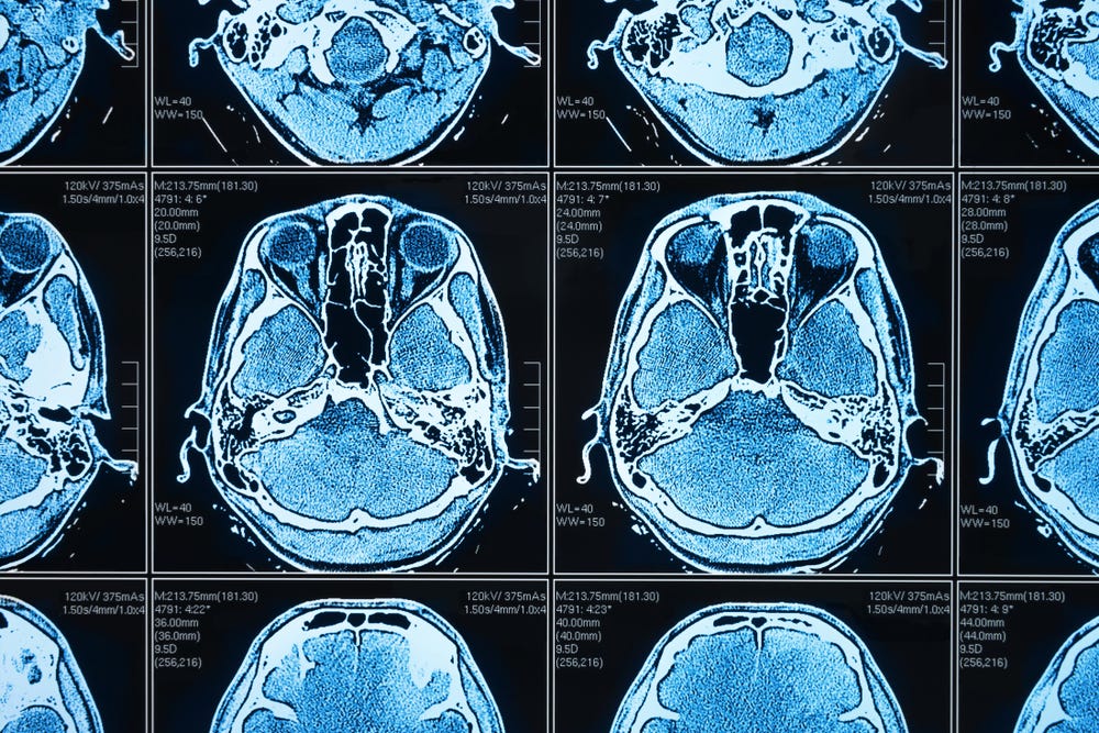
We like to thank Brad Genereaux, Prerna Dogra, Kristopher Kersten, Ahmed Harouni, and Wenqi Li from NVIDIA and the MONAI team for their active support in the development of this asset.
Since December 2021, we have released several examples to support Medical Imaging with Azure Machine Learning, and the response we received was overwhelming. The interest and inquiries reinforce how AI is quickly becoming a crucial aspect of modern medical practice.

3D Brain tumor segmentation use case
Today, we introduce a new medical imaging asset for 3D brain tumor segmentation, a solution that tackles a challenging use case in the field of oncology. Our solution leverages volumetric visual input from multiple MRI modalities and different 3D glioma tumor segmentations to produce accurate predictions of tumor boundaries and sub-regions. To handle the high amount of image data involved in this task, our asset employs parallel training using scalable GPU resources on Azure ML. Furthermore, we leverage the Medical Open Network for Artificial Intelligence (MONAI), a domain-specific framework that provides state-of-the-art tools and methods for medical image analysis.
Combining Azure Machine Learning and MONAI provides valuable synergies for scalable ML development and operations with specific innovations for medical imaging:
Azure Machine Learning is a cloud-based platform that provides a collaborative environment for data scientists and ML engineers to develop and deploy machine learning models at scale. It offers a range of authoring options, from no-code/low-code Automated ML to code-first using popular tools like VSCode. Users have access to scalable compute resources for training and deployment, making it ideal for handling large datasets and complex models. Additionally, it includes MLOps capabilities that enable the management and maintenance and versioning of ML assets, and allows for automated training and deployment pipelines. The platform includes responsible AI tools that can help explain models and mitigate potential bias, making it an ideal choice for businesses looking to develop and deploy ethical AI solutions.
The Medical Open Network for Artificial Intelligence (MONAI) is an open-source PyTorch-based project designed for medical imaging. It provides a comprehensive set of tools for building and deploying AI models for healthcare imaging:
- MONAI Label for AI-assisted labeling medical imaging data
- MONAI Core for training AI models with domain-specific capabilities
- MONAI Deploy for packaging, testing, and deploying medical AI applications.
MONAI Core is the focus of the solution described in this article. It offers native support for commonly used medical imaging formats such as Nifty and DICOM. It also includes features such as dictionary transforms that ensure consistency between images and segmentations in complex transformation pipelines. Moreover, MONAI Core provides a portfolio of network architectures, including state-of-the-art transformer-based 3D segmentation algorithms like UNETR.
Feel free to explore our demo and use it as a template for your own 3D segmentation use cases in (or beyond) medical domains.
We are using the 2021 version of the Brain Tumor Segmentation (BraTS) Challenge dataset. It is a collection of expert-annotated multimodal 3D magnetic resonance imaging (MRI) scans of brain tumors from different institutions. MRI is a medical imaging technique that uses a combination of magnetic fields and radio waves to visualize the internal structures of the body. Different MRI modalities can be generated by altering the imaging parameters, which results in varying tissue contrasts, making certain features more prominent in the images. The BraTS dataset uses the following modalities:
- Native T1 (T1): Can be used to differentiate between various tissue types and pathological conditions. T1 native is often used to extract quantitative information about tissue properties.
- T1-weighted with contrast agent Gadolinium (T1Gd): This modality can be used for delineating tumor boundaries and identifying areas of active tumor growth.
- T2-weighted (T2): These images are useful for detecting edema (fluid accumulation), inflammation, and other changes in brain tissue that may be associated with tumors.
- T2-weighted Fluid-Attenuated Inversion Recovery (T2-FLAIR): T2-FLAIR images are useful for identifying infiltrative tumor margins and non-enhancing tumor components.
The following illustration provides an example of the expert-annotated tumor segmentations available with the BraTS dataset: Tumor core, whole tumor, and enhancing structure. The image in the upper left corner combines the three segmentations.
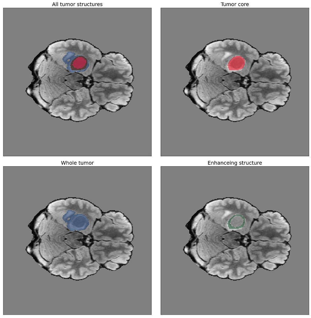
Being able to distinguish between these structures is critical for diagnosis, prognosis, and treatment planning. In the BraTS dataset, the whole tumor refers to the complete volume of the tumor, including the core and any surrounding edema or swelling. The core is the region within the tumor that contains the most aggressive cancer cells, known as the necrotic and active tumor. The enhancing structure refers to the region of the tumor that appears bright and enhances with contrast on MRI scans. This region is associated with the most active and invasive cancer cells.
Bringing it to action
Now, that we have gained an overview about the use case, let’s see how we are using Azure Machine Learning and MONAI to train and deploy a machine learning model for this interesting task.
The end-to-end workflow of this use case is implemented in our orchestration notebook. These are the main steps and their associated outputs:

The first steps involve downloading and visualizing the data, followed by submitting a training job to an Azure ML Compute Cluster. Once the model is trained and registered, it is deployed as an Azure ML Managed Endpoint. The notebook concludes with visualizing model predictions on an image volume from the validation set. The training and inferencing scripts are stored separately in the repository.
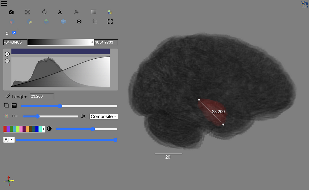
To manage machine learning assets like datasets, compute resources, experiments and the resulting model in our workflow, we use the Azure ML SDK to create a connection to the Azure ML Workspace. This connection can be established from any Python environment and does not require an Azure ML Compute Instance to run the code. By managing the assets with Azure ML, they can be found in the Azure ML Studio for future reference. This facilitates easy comparison between different experiments and creates a lineage for the resulting model by referencing the associated assets (dataset version, training code, environment etc.).
The data is downloaded from Kaggle using the Kaggle API and registered as an Azure ML managed dataset. This helps with versioning the training data, which is especially helpful in an iterative model development scenario where the training data may change over time. For instance, the BraTS dataset has been updated continuously since 2012. Linking the data version to a model ensures good governance.
The training script uses the MONAI framework along with native PyTorch classes. The data is pre-processed using several transforms provided by the MONAI framework, mainly using the dictionary-based wrappers. The different MRI modalities of the training images are stored as separate files and there is one file for the segmentation masks. The dictionary-based wrappers enable using a single pre-processing pipeline for all training data, where every transformation in the pipeline can be specified to which part of the data it should be applied.
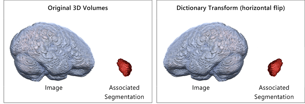
The following example illustrates the benefit of MONAI dictionary transforms to ensure consistency between the image and the associated segmentation labels. Imagine we use a pipeline of random transforms for data augmentation that affect the shape or position of the images (resize, flip, rotation, adjustment of perspective etc.). We have to make sure that the identical transformations are applied to the segmentation images to ensure consistency between images and labels for the downstream training process. MONAI dictionary transforms are a handy tool in this scenario: We simply need to specify if a transform should be applied to the image, the label or both. In this example, we will apply the transformations to both objects. MONAI also ensures consistency in the case of random transformations.
MONAI provides a portfolio of PyTorch based network architectures. We have chosen SegResNet (a variant of the ResNet architecture adapted for segmentation tasks) for our task. It is based on an encoder-decoder framework, where the encoder extracts features from the input image and the decoder reconstructs the output segmentation mask.
# Specify SegResNet for 3D segmentation
segresnet = SegResNet(
    blocks_down=[1, 2, 2, 4],
    blocks_up=[1, 1, 1],
    init_filters=16,
    in_channels=4,
    out_channels=3,
    dropout_prob=0.2,
).to(device)

# Wrap network for DDP
model = torch.nn.parallel.DistributedDataParallel(module=segresnet, device_ids=[local_rank])

# Specify Dice loss, optimizer and LR scheduler
loss_function = DiceLoss(smooth_nr=0, smooth_dr=1e-5, squared_pred=True, to_onehot_y=False, sigmoid=True)
optimizer = torch.optim.Adam(model.parameters(), initial_lr, weight_decay=1e-5)
lr_scheduler = torch.optim.lr_scheduler.CosineAnnealingLR(optimizer, T_max=max_epochs)
The number of encoder blocks for downsampling is specified by the blocks_down parameter. Accordingly, the upsampling blocks of the decoder part are defined with the blocks_up parameter. 16 filters are used in the first convolutional layer. The number is typically doubled as the network goes deeper, allowing it to learn more complex features. The network accepts input with 4 channels, specified by in_channels=4. This represents our multi-modal MRI data, where each channel corresponds to a different MRI modality: T1, T1Gd, T2 and T2-FLAIR. The output of the network has 3 channels, as specified by out_channels=3. This corresponds to our segmentation task classes of whole tumor, tumor core and enhancing structure.
PyTorch native features are used to include support for Distributed Data Parallel (DDP) training with multiple GPUs.
For the loss function, we leverage the Dice loss from MONAI. It is a common loss function used to measure the similarity between the predicted segmentation and the ground truth. It is particularly useful for problems with imbalanced class distributions, such as medical image segmentation, where the target region (e.g., tumor) is usually much smaller than the background.
The Adam optimizer is used in conjunction with a cosine annealing learning rate scheduler (CosineAnnealingLR). The scheduler oscillates the learning rate between an initial value and the specified minimum rate. CosineAnnealingLR can help improve model performance by allowing it to escape local minima during the initial stages of training and enabling precise adjustments in the later stages.
The training script is submitted to an Azure ML Compute Cluster via a Command Job, using the definition as follows:
job= command(
    inputs= {"input_data": Input(type=AssetTypes.URI_FOLDER, path= dataset_asset.path)},
    code= 'src/',
    command= "python train-brats21.py --epochs 50 --initial_lr 0.00025 --train_batch_size 1 --val_batch_size 1 --input_data $ --best_model_name BRATS21",
    environment= "monai-multigpu-azureml@latest",
    compute= train_target,
    experiment_name= experiment,
    display_name= f"3d brain tumor segmentation based on BRATS21",
    description= "## Brain tumor segmentation on 3D MRI brain scans",
    shm_size= '300g',
    resources= dict(instance_count= 1), # cluster nodes
    distribution= dict(type="PyTorch", process_count_per_instance= 4), # GPUs per node
    environment_variables= dict(AZUREML_ARTIFACTS_DEFAULT_TIMEOUT = 1000),
    services= {
    "My_jupyterlab": JobService(job_service_type="jupyter_lab"),
    "My_vscode": JobService(job_service_type="vs_code",),
    "My_tensorboard": JobService(job_service_type="tensor_board",),
        })

returned_job= ml_client.create_or_update(job)
When we submit the training job, a container is spun up in the Compute Cluster using the environment “monai-multi-gpu” that we defined earlier in the notebook. This environment is built from a conda specification file which contains the requirements for the training script. The resulting Docker image is cached in the Azure Container Registry that is linked to the Azure ML Workspace.
By using the distribution parameter, we initiate the number of processes as part of the distributed data parallel training. Since we used a machine with four GPUs for this experiment, we initiate four processes, each with access to their own GPU instance. Additionally, we can parallelize the training run over different nodes of the Compute Cluster by using the resources parameter.
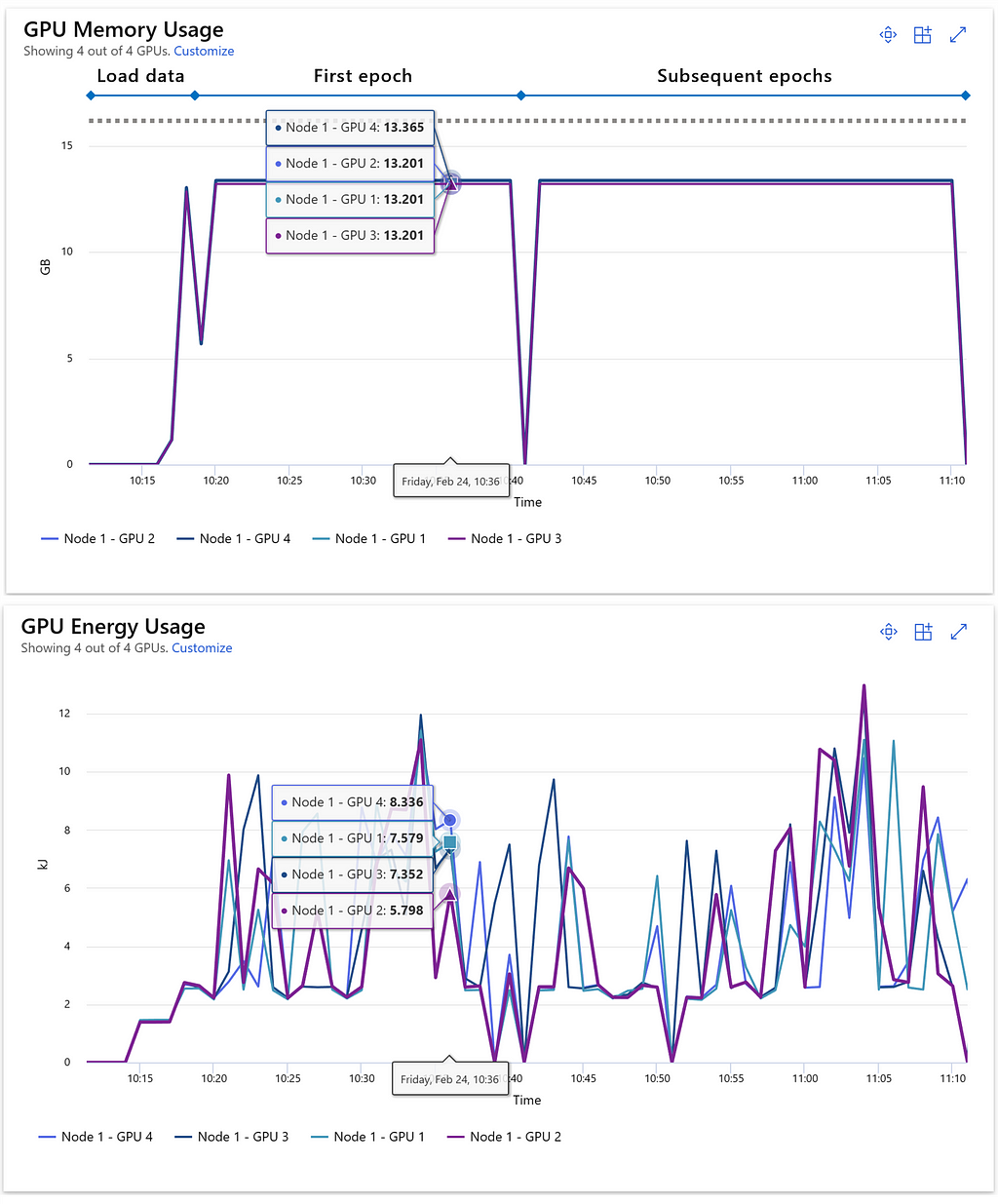
Understanding GPU utilization is crucial for optimizing resource usage and preventing the dreaded Out of Memory (OOM) errors that can occur during lengthy PyTorch training runs. Azure ML offers a range of metrics to track network and disk I/O, as well as CPU and GPU memory and processor utilization for active jobs. The following example demonstrates GPU memory and energy consumption at the start of a training run on a multi-GPU cluster node of the Standard_NC24rs_v3 type. In this scenario, we can see that the 16 GB of memory available on each of the four GPUs is being effectively utilized. There is only small headroom remaining, which makes clear that increasing the batch size could heighten the risk of encountering OOM errors. Additionally, Azure ML allows us to monitor the energy consumption of each GPU, measured in kilojoules.
Training with extensive datasets can require a significant amount of time, potentially taking several hours or even days to complete. The benefit of using a cloud-based data science and machine learning platform like Azure ML lies in the ability to access powerful resources on-demand as needed.
For our final model, we utilized NC96ads_A100_v4 cluster nodes with 96 cores, 880 GB of CPU memory, and 80 GB of memory for each of the four NVIDIA A100 GPUs to train over 150 epochs. The primary advantage of this setup is the on-demand availability of powerful resources: once training is complete, the cluster automatically shuts down, eliminating any further costs.
In our case, we opted for a “low priority” SKU, which offers a more cost-effective solution compared to dedicated compute resources. However, this choice comes with the risk of a running training job being preempted if the compute resources are required for other tasks.
While the training job is running, JupyterLab, VSCode, and Tensorboard are executed in the container, which makes it accessible for monitoring and debugging purposes. This is specified in the services parameter. We use Tensorboard and MLFlow logging in the training script to track training metrics, and MLFlow to register the final model. Both the metrics and model can be found as part of the experiment in the Azure ML Studio due to the native MLFlow support in Azure ML. By accessing the Tensorboard instance running on the container, we can review training and validation metrics while our model is trained.

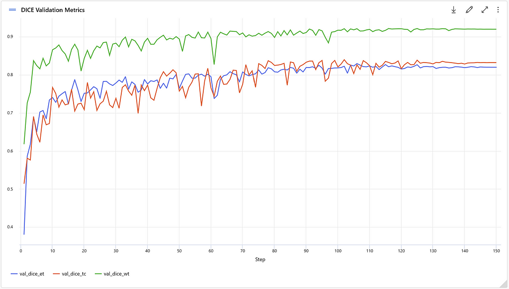
The Dice coefficient is used to evaluate model performance, which is a commonly used metric for object segmentation models. It measures the similarity between the predicted segmentation mask and the ground truth mask. A Dice coefficient of 1.0 indicates a perfect overlap between the predicted and the ground truth masks. Separate Dice metrics are tracked for the different classes in the dataset: Tumor core (val_dice_tc), whole tumor (val_dice_wt) and enhancing structure (val_dice_et). The average Dice metric across the different classes is also tracked (val_mean_dice). Running an experiment with 150 epochs results in the following metrics:
After registering the model, we move on to the deployment, which is a way to make the model accessible for predicting segmentation masks on new MRI images in a production setting. A possible deployment scenario for brain tumor segmentation is to integrate it with an MRI image viewer for diagnostic assistance. In the notebook, Azure ML Managed Endpoints are leveraged for deployment. First, a Managed Online Endpoint is created, which provides an interface for sending requests and receiving the inference output of a model. It also provides authentication and monitoring capabilities. Then, we create a deployment by defining the model, scoring script, environment, and target compute type. We reference the latest registered BraTS model in the Workspace for this deployment.
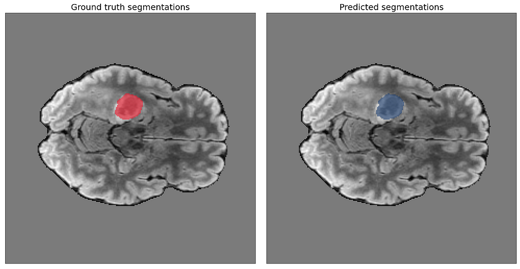
After sending a binary encoded version of the four modalities for a stack of MRI images to our endpoint, we receive predicted segmentations as part of the JSON response. The final part of the orchestration notebook contains code to visualize these predictions. Our image slider shows the predicted segmentations for each slice side by side with the ground truth to compare them.
Responsible use of AI in Healthcare
Incorporating machine learning into clinical practices, such as tumor detection and analysis, offers numerous benefits. For instance, algorithms can assist radiologists by flagging suspicious areas in the myriad of images generated daily. Another application involves the consistent monitoring of tumor progression to evaluate the effectiveness of cancer treatments. Manually calculating tumor volume from a collection of over a hundred slices per patient study can be incredibly time-consuming, but AI-assisted measurements can significantly expedite the process.
Despite the substantial advancements in AI-assisted image analysis, errors can still occur. Undetected tumors pose a considerable concern, and rare tumors or underrepresented patient characteristics in the training data can contribute to such false negatives. Consequently, it is crucial to address these limitations by incorporating diverse datasets and continuously refining the algorithms.
Physicians must continue to hold responsibility for diagnoses and treatment decisions. Machine learning predictions should be viewed as valuable and supportive tools, but not as infallible replacements for human expertise. The physician remains at the forefront of the entire process, ensuring that patient care is informed by both technology and professional judgment.
Conclusion
In this article, we explored the use of Azure Machine Learning and MONAI for 3D brain tumor segmentation, a challenging use case in the field of oncology. We discussed the various modalities of MRI images and the importance of distinguishing between tumor core, whole tumor, and enhancing structure for diagnosis, prognosis, and treatment planning. We also outlined the end-to-end workflow of this use case, including data visualization, training and registration of the model, deployment, and visualization of model predictions. The use of Azure Machine Learning and MONAI allowed us to employ parallel training using scalable GPU resources and provided domain-specific capabilities for training AI models for healthcare imaging.
We hope that our asset can serve as a template for future 3D segmentation use cases in medical domains and contribute to the growing importance of AI in modern medical practice.
The training code of this asset is based on an earlier version of the MONAI tutorial for 3D Brain Tumor Segmentation.
References
[1]: Hatamizadeh, A., Nath, V., Tang, Y., Yang, D., Roth, H. and Xu, D., 2022. Swin UNETR: Swin Transformers for Semantic Segmentation of Brain Tumors in MRI Images. arXiv preprint arXiv:2201.01266.
[2]: Tang, Y., Yang, D., Li, W., Roth, H.R., Landman, B., Xu, D., Nath, V. and Hatamizadeh, A., 2022. Self-supervised pre-training of swin transformers for 3d medical image analysis. In Proceedings of the IEEE/CVF Conference on Computer Vision and Pattern Recognition (pp. 20730–20740).
[3] U.Baid, et al., The RSNA-ASNR-MICCAI BraTS 2021 Benchmark on Brain Tumor Segmentation and Radiogenomic Classification, arXiv:2107.02314, 2021.
[4] B. H. Menze, A. Jakab, S. Bauer, J. Kalpathy-Cramer, K. Farahani, J. Kirby, et al. “The Multimodal Brain Tumor Image Segmentation Benchmark (BRATS)”, IEEE Transactions on Medical Imaging 34(10), 1993–2024 (2015) DOI: 10.1109/TMI.2014.2377694
[5] S. Bakas, H. Akbari, A. Sotiras, M. Bilello, M. Rozycki, J.S. Kirby, et al., “Advancing The Cancer Genome Atlas glioma MRI collections with expert segmentation labels and radiomic features”, Nature Scientific Data, 4:170117 (2017) DOI: 10.1038/sdata.2017.117
[6] S. Bakas, H. Akbari, A. Sotiras, M. Bilello, M. Rozycki, J. Kirby, et al., “Segmentation Labels and Radiomic Features for the Pre-operative Scans of the TCGA-GBM collection”, The Cancer Imaging Archive, 2017. DOI: 10.7937/K9/TCIA.2017.KLXWJJ1Q
Multimodal 3D Brain Tumor Segmentation with Azure ML and MONAI was originally published in Towards Data Science on Medium, where people are continuing the conversation by highlighting and responding to this story.
from Towards Data Science - Medium
https://towardsdatascience.com/multimodal-3d-brain-tumor-segmentation-with-azure-ml-and-monai-4a721e42f5f7?source=rss----7f60cf5620c9---4
via RiYo Analytics

No comments