https://ift.tt/qGsI07Y Better approaches to making statistical decisions Photo by Rommel Davila on Unsplash In establishing statistic...
Better approaches to making statistical decisions

In establishing statistical significance, the p-value criterion is almost universally used. The criterion is to reject the null hypothesis (H0) in favour of the alternative (H1), when the p-value is less than the level of significance (α). The conventional values for this decision threshold include 0.05, 0.10, and 0.01.
By definition, the p-value measures how compatible the sample information is with H0: i.e., P(D|H0), the probability or likelihood of data (D) under H0. However, as made clear from the statements of the American Statistical Association (Wasserstein and Lazar, 2016), the p-value criterion as a decision rule has a number of serious deficiencies. The main deficiencies include
- the p-value is a decreasing function of sample size;
- the criterion completely ignores P(D|H1), the compatibility of data with H1; and
- the conventional values of α (such as 0.05) are arbitrary with little scientific justification.
One of the consequences is that the p-value criterion frequently rejects H0 when it is violated by a practically negligible margin. This is especially so when the sample size is large or massive. This situation occurs because, while the p-value is a decreasing function of sample size, its threshold (α) is fixed and does not decrease with sample size. On this point, Wasserstein and Lazar (2016) strongly recommend that the p-value be supplemented or even replaced with other alternatives.
In this post, I introduce a range of simple, but more sensible, alternatives to the p-value criterion which can overcome the above-mentioned deficiencies. They can be classified into three categories:
- Balancing P(D|H0) and P(D|H1) (Bayesian method);
- Adjusting the level of significance (α); and
- Adjusting the p-value.
These alternatives are simple to compute, and can provide more sensible inferential outcomes than those solely based on the p-value criterion, which will be demonstrated using an application with R codes.
Background
Consider a linear regression model
Y = β0 + β1 X1 + … + βk Xk + u,
where Y is the dependent variable, X’s are independent variables, and u is a random error term following a normal distribution with zero mean and fixed variance. We consider testing for
H0: β1 = … = βq = 0,
against H1 that H0 does not hold (q ≤ k). A simple example is H0: β1 = 0; H1: β1 ≠ 0, where q =1.
Borrowing from the Bayesian statistical inference, we define the following probabilities:
Prob(H0|D): posterior probability for H0, which is the probability or likelihood of H0 after the researcher observes the data D;
Prob(H1|D) ≡ 1 — Prob(H0|D): posterior probability for H1;
Prob(D|H0): (marginal) likelihood of data under H0;
Prob(D|H1): (marginal) likelihood of data under H1;
P(H0): prior probability for H0, representing the researcher’s belief about H0 before she observes the data;
P(H1) = 1- P(H0): prior probability for H1.
These probabilities are related (by Bayes rule) as
The main components are as follows:
P10: the posterior odds ratio for H1 over H0, the ratio of the posterior probability of H1 to that of H0;
B10 ≡ P(D|H1)/P(D|H0) called the Bayes factor, the ratio of the (marginal) likelihood under H1 to that of H0;
P(H1)/P(H0): prior odds ratio.
Note that the posterior odds ratio is the Bayes factor multiplied by the prior odds ratio, and that that P10 = B10 if Prob(H0) = Prob(H1) = 0.5.
The decision rule is, if P10 > 0, the evidence favours H1 over H0. This means that, after the researcher observes the data, she favours H1 if P(H1|D) > P(H0|D), i.e., if the posterior probability of H1 is higher than that of H0.
For B10, the decision rule proposed by Kass and Raftery (1995) is given below:
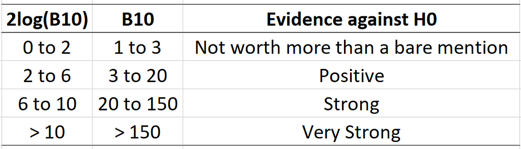
For example, if B10 = 3, then P(D|H1) = 3 × P(D|H0), which means that the data is compatible with H1 three times more than it is compatible with H0. Note that the Bayes factor is sometimes expressed as 2log(B10), where log() is the natural logarithm, in the same scale as the likelihood ratio test statistic.
Formulae for the alternatives
Bayes factor
Wagenmakers (2007) provides a simple approximation formula for the Bayes factor given by
2log(B10) = BIC(H0) — BIC(H1),
where BIC(Hi) denotes the value of the Bayesian information criterion under Hi (i = 0, 1).
Posterior probabilities
Zellner and Siow (1979) provide a formula for P10 given by
where F is the F-test statistic for H0, Γ() is the gamma function, v1 = n-k0-k1–1, n is the sample size, k0 is the number of parameters restricted under H0; and k1 is the number of parameters unrestricted under H0 (k = k0+k1).
Startz (2014) provides a formula for P(H0|D), posterior probability for H0, to test for H0: βi = 0:
where t is the t-statistic for H0: βi = 0, ϕ() is the standard normal density function, and s is the standard error estimator for the estimation of βi.
Adjustment to the p-value
Good (1988) proposes the following adjustment to the p-value:
where p is the p-value for H0: βi = 0. The rule is obtained by considering the convergence rate of the Bayes factor against a sharp null hypothesis. The adjusted p-value (p1) increases with sample size n.
Harvey (2017) proposes what is called the Bayesianized p-value
where PR ≡ P(H0)/P(H1) and MBF = exp(-0.5t²) is the minimum Bayes factor while t is the t-statistic.
Significance level adjustment
Perez and Perichhi (2014) propose an adaptive rule for the level of significance derived by reconciling the Bayesian inferential method and likelihood ratio principle, which is written as follows:
where q is number of parameters under H0, α is the initial level of significance such as 0.05, and χ²(α,q) is the α-level critical value from the chi-square distribution with q degrees of freedom. In short, the rule adjusts the level of significance as a decreasing function of sample size n.
Application with R Codes
In this section, we apply the above alternative measures to a regression with a large sample size, and examine how the inferential results are different from those obtained solely based on the p-value criterion. The R codes for the calculation of these measures are also provided.
Kamstra et al. (2003) examine the effect of depression linked with seasonal affective disorder on stock return. They claim that the length of sunlight can systematically affect the variation in stock return. They estimate the regression model of the following form:
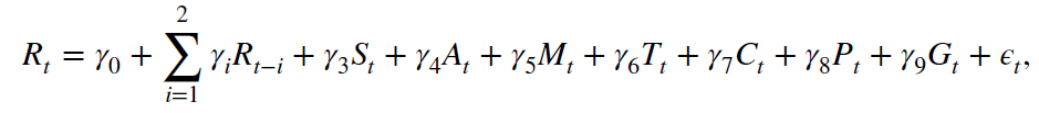
where R is the stock return in percentage on day t; M is a dummy variable for Monday; T is a dummy variable for the last trading day or the first five trading days of the tax year; A is a dummy variable for autumn days; C is cloud cover, P is precipitation; G is temperature, and S measures the length of sunlights.
They argue that, with a longer sunlight, investors are in a better mood, and they tend to buy more stocks which will increase the stock price and return. Based on this, their null and alternative hypotheses are
H0: γ3 = 0; H1: γ3 ≠ 0.
Their regression results are replicated using the U.S. stock market data, daily from Jan 1965 to April 1996 (7886 observations). The data range is limited by the cloud cover data which is available only from 1965 to 1996. The full results with further details are available from Kim (2022).
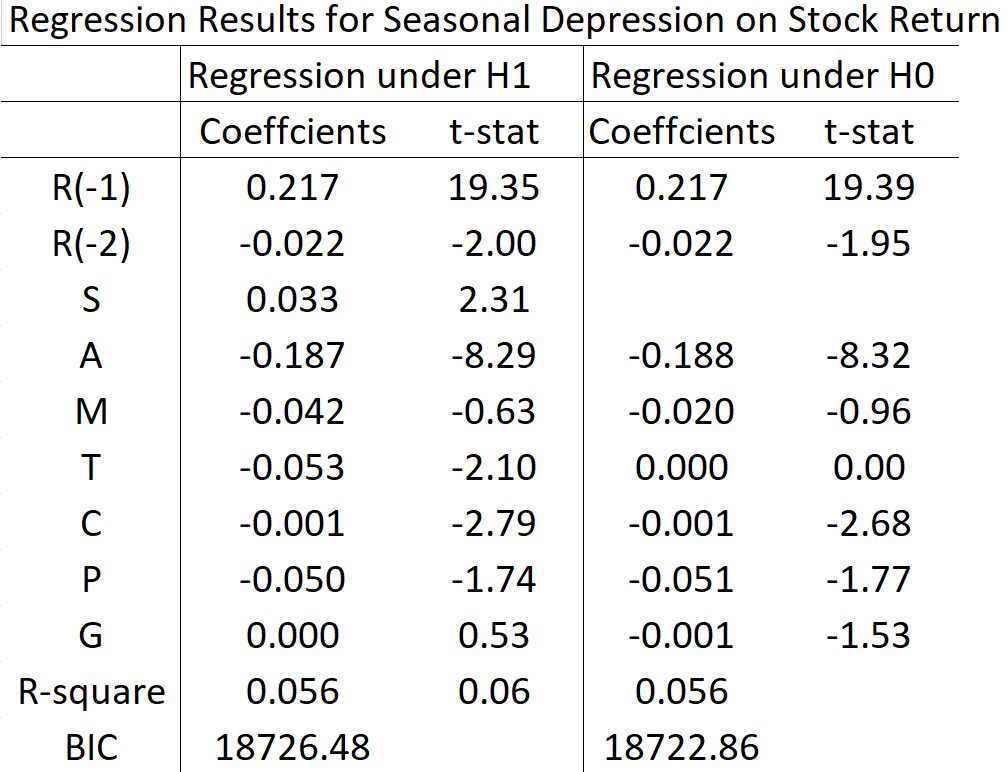
The above table presents a summary of the regression results under H0 and H1. The null hypothesis H0: γ3 = 0 is rejected at the 5% level of significance, with the coefficient estimate of 0.033, t-statistic of 2.31, and p-value of 0.027. Hence, based on the p-value criterion, the length of sunlight affects the stock return with statistical significance: the stock return is expected to increase by 0.033% in response to a 1-unit increase in the length of sunlight.
While this is evidence against the implications of stock market efficiency, it may be argued that whether this effect is large enough to be practically important is questionable.
The values of the alternative measures and the corresponding decisions are given below:
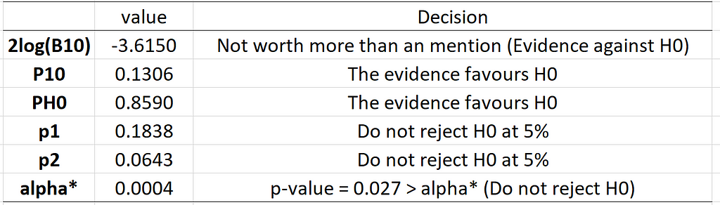
Note that P10 and p2 are calculated under the assumption that P(H0)=P(H1), which means that the researcher is impartial between H0 and H1 a priori. It is clear from the results in the above table that all of the alternatives to the p-value criterion strongly favours H0 over H1 or cannot reject H0 at the 5% level of significance. Harvey’s (2017) Bayesianized p-value that indicates rejection of H0 at the 10% level of significance.
Hence, we may conclude that the results of Kamstra et al. (2003), based solely on the p-value criterion, are not so convincing under the alternative decision rules. Given the questionable effect size and nearly negligible goodness-of-fit of the model (R² = 0.056), the decisions based on these alternatives seem more sensible.
The R code below shows the calculation of these alternatives (the full code and data are available from the author on request):
# Regression under H1
Reg1 = lm(ret.g ~ ret.g1+ret.g2+SAD+Mon+Tax+FALL+cloud+prep+temp,data=dat)
print(summary(Reg1))
# Regression under H0
Reg0 = lm(ret.g ~ ret.g1+ret.g2+Mon+FALL+Tax+cloud+prep+temp, data=dat)
print(summary(Reg0))

# 2log(B10): Wagenmakers (2007)
print(BIC(Reg0)-BIC(Reg1))

# PH0: Startz (2014)
T=length(ret.g); se=0.014; t=2.314
c=sqrt(2*3.14*T*se^2);
Ph0=dnorm(t)/(dnorm(t) + se/c)
print(Ph0)

# p-valeu adjustment: Good (1988)
p=0.0207
P_adjusted = min(c(0.5,p*sqrt(T/100)))
print(P_adjusted)


# Bayesianized p-value: Harvey (2017)
t=2.314; p=0.0207
MBF=exp(-0.5*t^2)
p.Bayes=MBF/(1+MBF)
print(p.Bayes)


# P10: Zellner and Siow (1979)
t=2.314
f=t^2; k0=1; k1=8; v1 = T-k0-k1- 1
P1 =pi^(0.5)/gamma((k0+1)/2)
P2=(0.5*v1)^(0.5*k0)
P3=(1+(k0/v1)*f)^(0.5*(v1-1))
P10=(P1*P2/P3)^(-1)
print(P10)

# Adaptive Level of Significance: Perez and Perichhi (2014)
n=T;alpha=0.05
q = 1                           # Number of Parameters under H0
adapt1 = ( qchisq(p=1-alpha,df=q) + q*log(n) )^(0.5*q-1)
adapt2 = 2^(0.5*q-1) * n^(0.5*q) * gamma(0.5*q)
adapt3 = exp(-0.5*qchisq(p=1-alpha,df=q))
alphas=adapt1*adapt3/adapt2
print(alphas)
Conclusion
The p-value criterion has a number of deficiencies. Sole reliance on this decision rule has generated serious problems in scientific research, including accumulation of wrong stylized facts, research integrity, and research credibility: see the statements of the American Statistical Association (Wasserstein and Lazar, 2016).
This post presents several alternatives to the p-value criterion for statistical evidence. A balanced and informed statistical decision can be made by considering the information from a range of alternatives. Mindless use of a single decision rule can provide misleading decisions, which can be highly costly and consequential. These alternatives are simple to calculate and can supplement the p-value criterion for better and more informed decisions.
Please Follow Me for more engaging posts!
Alternatives to the p-value Criterion for Statistical Significance (with R code) was originally published in Towards Data Science on Medium, where people are continuing the conversation by highlighting and responding to this story.
from Towards Data Science - Medium
https://towardsdatascience.com/alternatives-to-the-p-value-criterion-for-statistical-significance-with-r-code-222cfc259ba7?source=rss----7f60cf5620c9---4
via RiYo Analytics


No comments