https://ift.tt/Eqi0PNM The classical inventory management optimization problem solved in Python using Pyomo Photo by CHUTTERSNAP on Uns...
The classical inventory management optimization problem solved in Python using Pyomo

Lot sizing problems are production planning problems with setups between production lots. By reason of these setups, it is often too costly to produce a given product in every period (Suwondo & Yuliando, 2012). In contrast, fewer setups are associated with higher holding inventory costs. Therefore, to obtain optimal costs, one should balance these operational aspects.
Throughout this article, the problem proposed by Wagner & Whitin (1958) will be implemented using a mixed-integer programming approach. To do so, the Python library pyomo (Bynum et al., 2021) will be used with the CBC solver. Personally, I find this problem extremely useful to introduce notions of inventory management in discrete planning horizons for numerical optimization, which is ubiquitous in more complex problems. Notice that, in their original work, Wagner & Whitin (1958) developed an exact algorithm for solving this problem, which differs from the approach herein adopted.
You can find the notebook with the complete implementation of the problem here.
If you are unfamiliar with numerical optimization and/or mixed-integer programming, you might want to see this introduction on the subject beforehand.
An introduction to mixed-integer linear programming: The knapsack problem
Problem statement
Suppose that, for a given horizon T of instants t, you can predict demands d for a given product for each t. Furthermore, consider you can predict setup costs s and inventory holding costs h for each time instant. If any amount of a product is produced in a given time t, the corresponding setup cost s should be incurred. Also, at the end of each period, holding inventory costs should be incurred, which correspond to h times the final inventory at t.
If the problem is uncapacitated, as considered in Wagner & Whitin (1958), one can state that every demand should be met. Moreover, consider that unitary production costs are not time-dependent, although small changes in the problem structure might easily introduce these costs. Your goal is to determine how many units of the product are produced at each instant so that we minimize setup and holding inventory costs.
I will describe each modeling component in detail in the next section, but the complete optimization problem considered can be summarized by the following equations.

Modeling
Let us start by importing the Python libraries used:
import numpy as np
import pandas as pd
import pyomo.environ as pyo
import matplotlib.pyplot as plt
And now, let us instantiate the dataset as in the example of the original article (Wagner & Whitin, 1958).
months = np.arange(12, dtype=int) + 1
setup_cost = np.array([85, 102, 102, 101, 98, 114, 105, 86, 119, 110, 98, 114])
demand = np.array([69, 29, 36, 61, 61, 26, 34, 67, 45, 67, 79, 56])
inventory = np.ones(12)

dataset = pd.DataFrame(
    {"setup_cost": setup_cost, "inventory_cost": inventory, "demand": demand},
    index=months,
)
As we are using Pyomo in this example, we must first instantiate the pyomo model. In this example, I chose to use the ConcreteModel approach as I find it more straightforward for simple problems. Alternatively, one could have used an AbstractModel. Both are described in more detail here.
model = pyo.ConcreteModel()
The only Set considered in this problem is the planning horizon T. Let us instantiate it as a pyomo object.
model.T = pyo.Set(initialize=list(dataset.index))
Next, we will instantiate model parameters imported from the problem dataset. They are the following:
- d: demand at each time t
- s: setup cost each time t
- h: holding inventory cost at each time t
model.d = pyo.Param(model.T, initialize=dataset.demand)
model.s = pyo.Param(model.T, initialize=dataset.setup_cost)
model.h = pyo.Param(model.T, initialize=dataset.inventory_cost)
And the decision variables:
- x: product amount produced at each time t
- y: binary variable that marks setup costs at each time t
- I: final inventory at each time t
model.x = pyo.Var(model.T, within=pyo.NonNegativeReals)
model.y = pyo.Var(model.T, within=pyo.Binary)
model.I = pyo.Var(model.T, within=pyo.NonNegativeReals)
The inventory balance constraint states that the inventory at the end of a period t is equal to the inventory at the end of the previous period plus the amount produced minus the demand at that given period. We consider here the initial inventory as equal to zero.

def inventory_rule(model, t):
    if t == model.T.first():
        return model.I[t] == model.x[t] - model.d[t]
    else:
        return model.I[t] == model.I[model.T.prev(t)] + model.x[t] - model.d[t]

model.inventory_rule = pyo.Constraint(model.T, rule=inventory_rule)
Now let us formulate the big M constraint to identify periods with setup costs. Our intention is that y should be 1 if any amount of the product is produced at time t and 0 otherwise.

In general, you might want to choose the smallest value of M that is large enough to avoid removing feasible solutions from the integer decision space. This might produce better best-bound values during the branch-and-bound algorithm than choosing arbitrarily large values.
In this problem, it only makes sense to produce a certain demand lot d at time t-n, if holding inventory costs from time t-n to t are lesser than or equal to setup costs at t. So we can calculate the “maximum intelligent production” at an instant t by the following lines:
def get_max_antecip(t, dataset=dataset):
    """
    Returns the first instant in which it might be
    intelligent to produce a certain demand
    """

    total_inv = 0
    d = dataset.demand[t]
    s = dataset.setup_cost[t]
    out = t

    for i in range(1, t - dataset.index[0] + 1):
        h = dataset.inventory_cost[t - i]
        if total_inv + h * d <= s:
            total_inv = total_inv + h * d
            out = t - i
        else:
            break

    return out


def get_max_prod(t, dataset=dataset):
    df = dataset.query(f"max_antecip <= {t} & index >= {t}")
    return df.demand.sum()


dataset["max_antecip"] = [get_max_antecip(t, dataset=dataset) for t in dataset.index]
dataset["max_prod"] = [get_max_prod(t, dataset=dataset) for t in dataset.index]
And now we can define a proper M value for each time period and instantiate the big M constraint.
model.M = pyo.Param(model.T, initialize=dataset.max_prod)

def active_prod(model, t):
    return model.x[t] <= model.M[t] * model.y[t]

model.active_prod = pyo.Constraint(model.T, rule=active_prod)
At last, the objective function sums all holding inventory and setup costs in the planning horizon.

def total_cost(model):
    holding = sum(model.h[t] * model.I[t] for t in model.T)
    setup = sum(model.s[t] * model.y[t] for t in model.T)
    return total_setup(model) + total_holding(model)

model.obj = pyo.Objective(rule=total_cost, sense=pyo.minimize)
To solve the model I used the open-source solver CBC. You can download CBC binaries from AMPL or this link. You can also find an installation tutorial here. As the CBC executable is included in the PATH variable of my system, I can instantiate the solver without specifying the path to an executable file. If yours is not, parse the keyword argument “executable” with the path to your executable file.
# executable=YOUR_PATH
solver = pyo.SolverFactory("cbc")
Alternatively, one could have used GLPK to solve this problem (or any other solver compatible with pyomo). The latest available GLPK version can be found here and the Windows executable files can be found here.
solver.solve(model, tee=True)
And we are done! The results are stored in our model and will be analyzed in detail in the next section.
Results
First, let us print the naive scenario costs, in which every demand should be produced in its corresponding instant.
# Obtain the maximum cost for comparison
max_cost = dataset.setup_cost.sum()
print(f"Maximum cost: {max_cost:.1f}")
Which should return 1234.0.
Next, let us obtain the new costs from the objective function and compare the results:
opt_value = model.obj()
print(f"Best cost {opt_value}")
print(f"% savings {100 * (1 - opt_value / max_cost) :.2f}")
Wow! The new cost is 864.0 and savings are almost 30%!
Let us include new columns in the dataset and plot production versus demand to visualize the results better:
# Include production as a column
dataset["production"] = [model.x[t].value for t in dataset.index]

# Plot figure
fig, ax = plt.subplots(figsize=[6, 3], dpi=100)
x = dataset.index
width = 0.35
ax.bar(x - width/2, dataset.production, width, color="darkgreen", label="production")
ax.bar(x + width/2, dataset.demand, width, color="navy", label="demand")
ax.set_xticks(x)
ax.set_ylabel("Qtd")
ax.set_xlabel("t")
ax.legend()
fig.tight_layout()
plt.show()
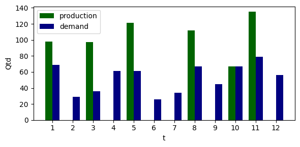
One can notice that, except for instant 10, which holds a single demand, other demands were combined in the same production instants so that the overall setup costs were significantly reduced.
Conclusions
In this article, the dynamic lot-size model (Wagner & Whitin, 1958) was formulated and solved as a mixed-integer programming problem. Compared to a naive solution, the optimization results would reduce overall costs by 30%. In this scenario, holding inventory and setup costs are adequately balanced. The complete solutions are available in this git repository.
Further reading
Those interested in more details about integer programming can refer to Wolsey (2020); for operations research, Winston & Goldberg (2004).
The Branch & Bound algorithm is the most used in the solution of integer and mixed-integer problems. Those interested in an introduction to its mechanisms can refer to my previous Medium article.
References
Bynum, M. L. et al., 2021. Pyomo-optimization modeling in python. Springer.
Suwondo, E., & Yuliando, H. (2012). Dynamic lot-sizing problems: a review on model and efficient algorithm. Agroindustrial journal, 1(1), 36.
Wagner, H. M., & Whitin, T. M. (1958). Dynamic version of the economic lot size model. Management science, 5(1), 89–96.
Winston, W. L. & Goldberg, J. B., 2004. Operations research: applications and algorithms. 4th ed. Belmont, CA: Thomson Brooks/Cole Belmont.
Wolsey, L. A., 2020. Integer Programming. 2nd ed. John Wiley & Sons.
The dynamic lot-size model: A mixed-integer programming approach was originally published in Towards Data Science on Medium, where people are continuing the conversation by highlighting and responding to this story.
from Towards Data Science - Medium
https://towardsdatascience.com/the-dynamic-lot-size-model-a-mixed-integer-programming-approach-4a9440ba124e?source=rss----7f60cf5620c9---4
via RiYo Analytics


No comments