https://ift.tt/th6K8Wc How to optimize the media mix using saturation curves and statistical models Photo by Joel Filipe on Unsplash ...
How to optimize the media mix using saturation curves and statistical models

Marketing Mix Modeling (MMM) is a data-driven approach that is used to identify and analyze the key drivers of the business outcome such as sales or revenue by examining the impact of various factors that may influence the response. The goal of MMM is to provide insights into how marketing activities, including advertising, pricing, and promotions, can be optimized to improve the business performance. Among all the factors influencing the business outcome, marketing contribution, such as advertising spend in various media channels, is considered to have a direct and measurable impact on the response. By analyzing the effectiveness of advertising spend in different media channels, MMM can provide valuable insights into which channels are the most effective for increasing sales or revenue, and which channels may need to be optimized or eliminated to maximize marketing ROI.
Short introduction into MMM
Marketing Mix Modeling (MMM) is a multi-step process involving series of unique steps that are driven by the marketing effects being analyzed. First, the coefficients of the media channels are constrained to be positive to account for positive effect of advertising activity.
Modeling Marketing Mix with Constrained Coefficients
Second, adstock transformation is applied to capture the lagged and decayed impact of advertising on consumer behavior.
Modeling Marketing Mix using PyMC3
Third, the relationship between advertising spend and the corresponding business outcome is not linear, and follows the law of diminishing returns. In most MMM solutions, the modeler typically employs linear regression to train the model, which presents two key challenges. Firstly, the modeler must apply the saturation transformation step to establish the non-linear relationship between the media activity variables and the response variable. Secondly, the modeler must develop hypotheses about the possible transformation functions that are applicable to each media channel. However, more complex machine learning models may capture non-linear relationships without applying the saturation transformation.
- Modeling Marketing Mix Using Smoothing Splines
- Improving Marketing Mix Modeling Using Machine Learning Approaches
The last step is to build a marketing mix model by estimating the coefficients, and parameters of the adstock and saturation functions.
Budget Optimization
Both saturation curves and a trained model can be used in marketing mix modeling to optimize budget spend. The advantages of using saturation curves are:
- Simplicity in visualizing the influence of spend on the outcome
- The underlying model is not required anymore so budget optimization procedure is simplified and requires only the parameters of the saturation transformation
One of the disadvantages is that saturation curves are based on historical data and may not always accurately predict the response to future spends.
The advantages of using the trained model for budget optimization is that the model uses complex relationship between media activities and other variables including trend, and seasonality and can better capture the diminishing returns over time.
Data
I continue using the dataset made available by Robyn under MIT Licence as in my previous articles for practical examples, and follow the same data preparation steps by applying Prophet to decompose trends, seasonality, and holidays.
The dataset consists of 208 weeks of revenue (from 2015–11–23 to 2019–11–11) having:
- 5 media spend channels: tv_S, ooh_S, print_S, facebook_S, search_S
- 2 media channels that have also the exposure information (Impression, Clicks): facebook_I, search_clicks_P (not used in this article)
- Organic media without spend: newsletter
- Control variables: events, holidays, competitor sales (competitor_sales_B)
Modeling
I built a complete working MMM pipeline that can be applied in a real-life scenario for analyzing media spend on the response variable, consisting of the following components:
- Adstock Transformation with infinite decay rate (0 < α < 1)
- Saturation Hill Transformation with two parameters: slope / shape parameter, controlling the steepness of the curve (s > 0) and half saturation point (0 < k ≤ 1)
- Ridge Regression from scikit-learn
- Time-based cross-validation
- Optuna hyperparameter tuning
A note on coefficients
In scikit-learn, Ridge Regression does not offer the option to set a subset of coefficients to be positive. However, a possible workaround is to reject the optuna solution if some of the media coefficients turn out to be negative. This can be achieved by returning a very large value, indicating that the negative coefficients are unacceptable and must be excluded.
A note on saturation transformation
The Hill saturation function assumes that the input variable falls within a range of 0 to 1, which means that the input variable must be normalized before applying the transformation. This is important because the Hill function assumes that the input variable has a maximum value of 1.
However, it is possible to apply the Hill transformation on non-normalized data by scaling the half saturation parameter to the spend range by using the following equation:
half_saturation_unscaled = half_saturation * (spend_max - spend_min) + spend_min
where half_saturation is the original half saturation parameter in the range between 0 and 1, spend_min and spend_max represent the minimum and maximum spend values, respectively.
The complete transformation function is provided below:
class HillSaturation(BaseEstimator, TransformerMixin):
    def __init__(self, slope_s, half_saturation_k):
        self.slope_s = slope_s
        self.half_saturation_k = half_saturation_k

    def fit(self, X, y=None):
        return self

    def transform(self, X: np.ndarray, x_point = None):

        self.half_saturation_k_transformed  = self.half_saturation_k * (np.max(X) - np.min(X)) + np.min(X)

        if x_point is None:
            return (1 + self.half_saturation_k_transformed**self.slope_s / X**self.slope_s)**-1

        #calculate y at x_point
        return (1 + self.half_saturation_k_transformed**self.slope_s / x_point**self.slope_s)**-1
Budget Optimization using Saturation Curves
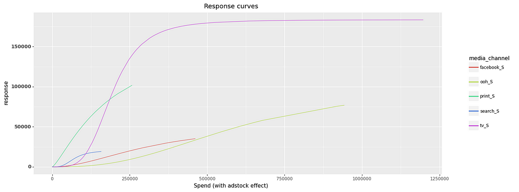
Once the model is trained, we can visualize the impact of media spend on the response variable using response curves that have been generated through Hill saturation transformations for each media channel. The plot below illustrates the response curves for five media channels, depicting the relationship between spend of each channel (on weekly basis) and response over a period of 208 weeks.

Optimizing budget using saturation curves involves identifying the optimal spend for each media channel that will result in the highest overall response while keeping the total budget fixed for a selected time period.
To initiate optimization, the average spend for a specific time period is generally used as a baseline. The optimizer then uses the budget per channel, which can fluctuate within predetermined minimum and maximum limits (boundaries), for constrained optimization.
The following code snippet demonstrates how budget optimization can be achieved using the minimize function from the scipy.optimize package. However, it’s worth noting that alternative optimization packages, such as nlopt or nevergrad, can also be used for this purpose.
optimization_percentage = 0.2

media_channel_average_spend = result["model_data"][media_channels].mean(axis=0).values

lower_bound = media_channel_average_spend * np.ones(len(media_channels))*(1-optimization_percentage)
upper_bound = media_channel_average_spend * np.ones(len(media_channels))*(1+optimization_percentage)

boundaries = optimize.Bounds(lb=lower_bound, ub=upper_bound)

def budget_constraint(media_spend, budget):
  return np.sum(media_spend) - budget


def saturation_objective_function(coefficients,
                                  hill_slopes,
                                  hill_half_saturations,
                                  media_min_max_dictionary,
                                  media_inputs):

    responses = []
    for i in range(len(coefficients)):
        coef = coefficients[i]
        hill_slope = hill_slopes[i]
        hill_half_saturation = hill_half_saturations[i]

        min_max = np.array(media_min_max_dictionary[i])
        media_input = media_inputs[i]

        hill_saturation = HillSaturation(slope_s = hill_slope, half_saturation_k=hill_half_saturation).transform(X = min_max, x_point = media_input)
        response = coef * hill_saturation
        responses.append(response)

    responses = np.array(responses)
    responses_total = np.sum(responses)
    return -responses_total


partial_saturation_objective_function = partial(saturation_objective_function,
                                                media_coefficients,
                                                media_hill_slopes,
                                                media_hill_half_saturations,
                                                media_min_max)


max_iterations = 100
solver_func_tolerance = 1.0e-10

solution = optimize.minimize(
      fun=partial_saturation_objective_function,
      x0=media_channel_average_spend,
      bounds=boundaries,
      method="SLSQP",
      jac="3-point",
      options={
          "maxiter": max_iterations,
          "disp": True,
          "ftol": solver_func_tolerance,
      },
      constraints={
          "type": "eq",
          "fun": budget_constraint,
          "args": (np.sum(media_channel_average_spend), )
      })
Some important points:
- fun — the objective function to be minimized. In this case, it takes the following parameters:
media coefficients — Ridge regression coefficients for each media channel that are multiplied with the corresponding saturation level to estimate the response level for each media channel.
slopes and half saturations — two parameters of the Hill transformation spend min-max values for each media channel to correctly estimate the response level for a given media spend.
The objective function iterates over all media channels and calculates the total response based on the sum of individual response levels per media channel. To maximize the response in the optimization function, we need to convert it into a minimization problem. Therefore, we obtain the negative value of the total response, which we then use as the objective for the optimization function. - method = SLSQP — The Sequential Least Squares Programming (SLSQP) algorithm is a popular method for constrained optimization problems, and it is often used for optimizing budget allocation in marketing mix modeling.
- x0 — Initial guess. Array of real elements of size (n,), where n is the number of independent variables. In this case, x0 corresponds to the media channel average spend, i.e., an array of average spends per channel.
- bounds — refers to the bounds of media spend per channel.
- constraints — constraints for SLSQP are defined as a list of dictionaries, where budget_constraint is a function that ensures that the sum of media spends is equal to the fixed budget: np.sum(media_channel_average_spend)
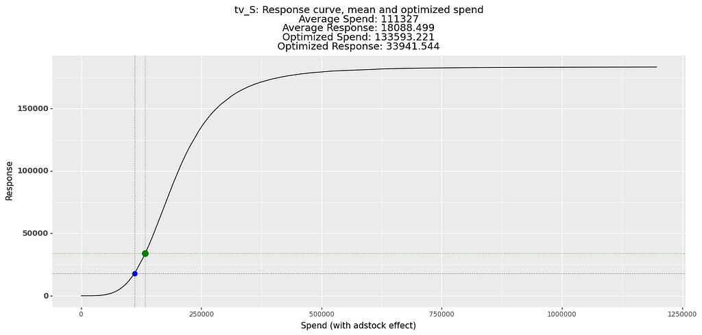
After the optimization process is complete, we can generate response curves for each media channel and compare the spend allocation before and after optimization to assess the impact of the optimization process.

Budget Optimization using the Trained Model
The process of optimizing the budget using the trained model is quite similar to the previous approach, and can be applied to both models that have and those that do not have the saturation transformation. This approach offers greater flexibility for optimizing marketing mix, allowing for optimization across various time periods, including future ones.
The following code highlights the differences between the current and the previous approach:
The average spend per channel is multiplied by the desired optimization period
optimization_period = result["model_data"].shape[0]
print(f"optimization period: {optimization_period}")


optimization_percentage = 0.2


media_channel_average_spend = optimization_period * result["model_data"][media_channels].mean(axis=0).values

lower_bound = media_channel_average_spend * np.ones(len(media_channels))*(1-optimization_percentage)
upper_bound = media_channel_average_spend * np.ones(len(media_channels))*(1+optimization_percentage)

boundaries = optimize.Bounds(lb=lower_bound, ub=upper_bound)
We can interpet the results of the optimization as “what is the appropriate amount of spending per channel during a specific time interval”
The objective function expects two additional parameters: optimization_periodand additional_inputs— all other variables like trend, seasonality, control variables used for model training and available for the selected time period:
def model_based_objective_function(model,
                                   optimization_period,
                                   model_features,
                                   additional_inputs,
                                   hill_slopes,
                                   hill_half_saturations,
                                   media_min_max_ranges,
                                   media_channels,
                                   media_inputs):

    media_channel_period_average_spend = media_inputs/optimization_period

    #transform original spend into hill transformed
    transformed_media_spends = []
    for index, media_channel in enumerate(media_channels):
        hill_slope = hill_slopes[media_channel]
        hill_half_saturation = hill_half_saturations[media_channel]

        min_max_spend = media_min_max_ranges[index]
        media_period_spend_average = media_channel_period_average_spend[index]

        transformed_spend = HillSaturation(slope_s = hill_slope, half_saturation_k=hill_half_saturation).transform(np.array(min_max_spend), x_point = media_period_spend_average)
        transformed_media_spends.append(transformed_spend)

    transformed_media_spends = np.array(transformed_media_spends)

    #replicate average perio spends into all optimization period
    replicated_media_spends = np.tile(transformed_media_spends, optimization_period).reshape((-1, len(transformed_media_spends)))

    #add _hill to the media channels
    media_channels_input = [media_channel + "_hill" for media_channel in media_channels]
    media_channels_df = pd.DataFrame(replicated_media_spends, columns = media_channels_input)


    #prepare data for predictions
    new_data = pd.concat([additional_inputs, media_channels_df], axis = 1)[model_features]

    predictions = model.predict(X = new_data)

    total_sum = predictions.sum()

    return -total_sum
The objective function takes in media spends that are bounded by our constraints within the time period through the media_inputs parameter. We assume that these media spends are equally distributed along all weeks of the time period. Therefore, we first divide media_inputs by the time period to obtain the average spend and then replicate it using np.tile.After that, we concatenate the non-media variables with the media spends and use them to predict the response withmodel.predict(X=new_data)for each week within the time interval. Finally, we calculate the total response as the sum of the weekly responses and return the negative value of the total response for minimization.
Conclusion
Optimizing budget spend in marketing mix modeling is important because it allows marketers to allocate their resources in the most effective way possible, maximizing the impact of their marketing efforts and achieving their business objectives.
I showed two practical approaches to optimizing marketing mix using saturation curves and trained models.
For a detailed implementation, please refer to the complete code available for download on my Github repo.
Thanks for reading!
Practical Approaches to Optimizng Budget in Marketing Mix Modeling was originally published in Towards Data Science on Medium, where people are continuing the conversation by highlighting and responding to this story.
from Towards Data Science - Medium
https://towardsdatascience.com/practical-approaches-to-optimizng-budget-in-marketing-mix-modeling-7816a27f2f71?source=rss----7f60cf5620c9---4
via RiYo Analytics

No comments