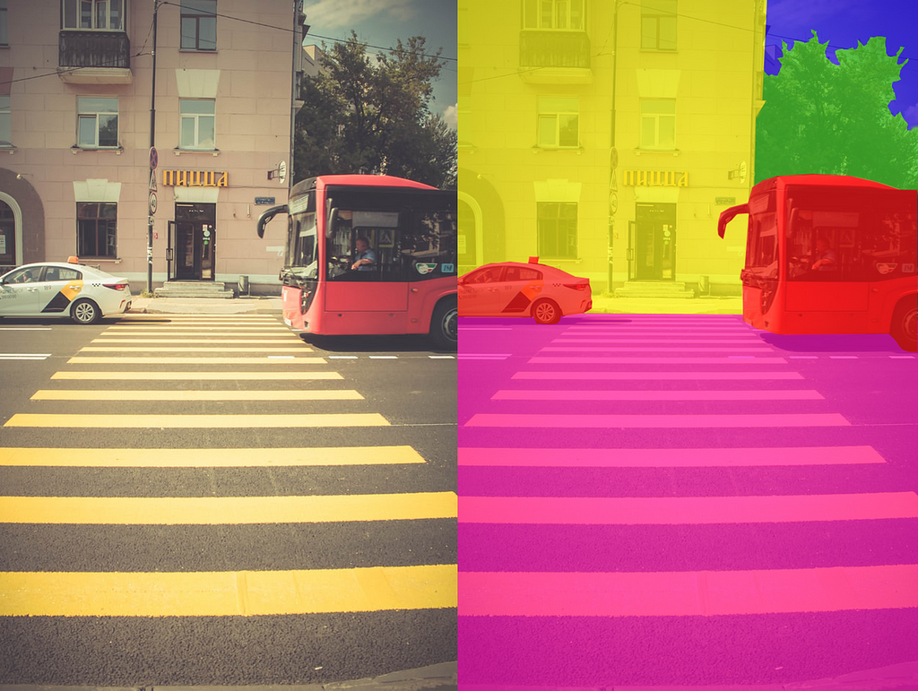
https://ift.tt/8aMrNFt Knowing various Computer Vision tasks and their formats Image Source: Wikimedia (Creative Commons) Introduction:...
Knowing various Computer Vision tasks and their formats

Introduction:
Computer Vision(CV) is the field that makes computers extract information from images like how the Human Visual System can do.
There are various Computer Vision tasks, all of which typically take an image of dimension WxHx3 as input and produce the output according to the task at hand. While H and W represent the image’s resolution (Height and Width), 3 is the number of channels (R, G, and B).
“The first step to solving a problem is to define it well.”
This article covers various Computer Vision tasks and their formats, defined mathematically, highlighting what the corresponding inputs and outputs for each task are.
Various Computer Vision tasks:
- Image Classification
- Binary Classification
- Multi-class Classification
- Multi-label Classification - Classification with Localization
- Object Detection
- Image Segmentation
- Semantic Segmentation
- Instance Segmentation
- Panoptic Segmentation
1. Image Classification:
Image Classification is the task of classifying or categorizing a given image into pre-defined classes.
Binary Classification:
Binary classification classifies a given image into either of the two pre-defined classes.
Input: X — Dimension: W x H x 3
Output: Y — Dimension: 1
Here, the ground truth value of an output Y will be either 1 or 0 (for positive and negative examples, respectively).
However, a binary classification model’s output will typically be a number between 0 and 1, which will be treated as a probability of the input image belonging to the positive class.

The below example classifies an input image into either ‘Cat’ or ‘Not a Cat.’

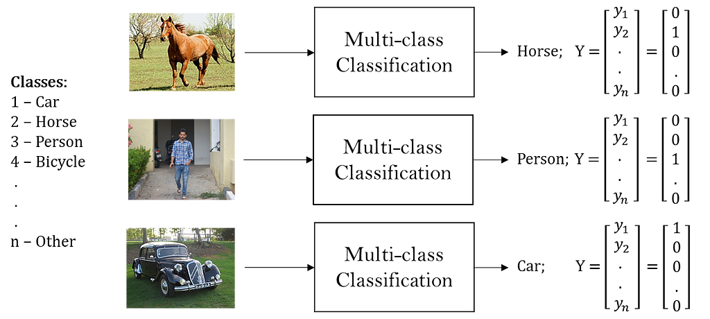
Multi-class Classification:
Multi-class classification classifies a given image into one among the many(n) pre-defined classes.
Input: X — Dimension: W x H x 3
Output: Y — Dimension: n x 1
Here, the ground truth value of an output Y will be a one-hot encoded vector (position of 1 indicating the class assigned to the input image).
However, a multi-class classification model’s output will typically be a vector of numbers between 0 and 1, all of which add up to 1. These will be treated as probabilities of the input image belonging to the respective classes.

The below example classifies an input image into one among the n pre-defined classes.

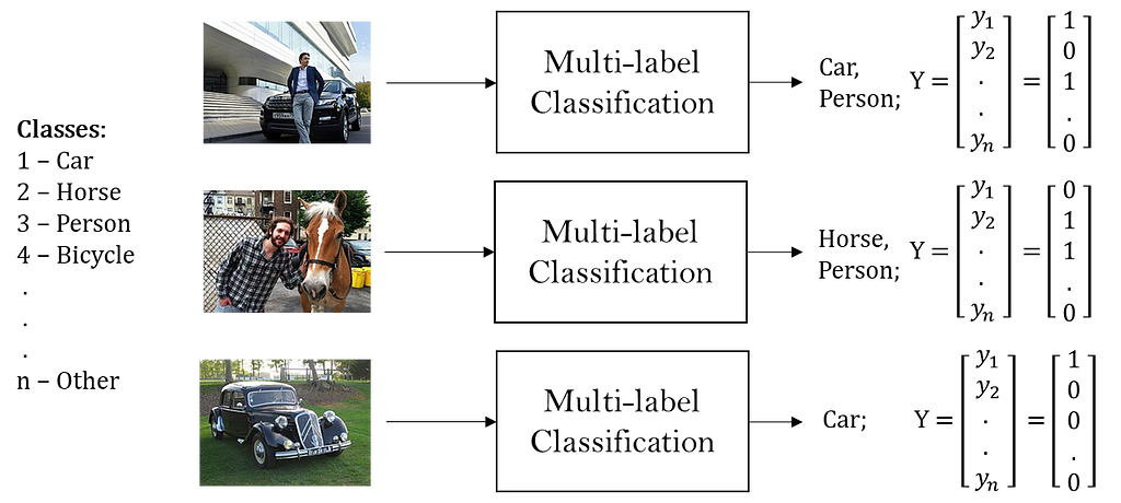
Multi-label Classification:
Multi-label classification is similar to multi-class classification except that the input image can be assigned with more than one pre-defined class among n.
Input: X — Dimension: W x H x 3
Output: Y — Dimension: n x 1
Here, the ground truth value of an output Y can have 1 in more than one position. So it can be a binary vector instead of a one-hot vector.
However, a multi-label classification model’s output will typically be a vector of numbers between 0 and 1. Note that these numbers need not add up to 1 since an input image can belong to more than one pre-defined class at a time. Each number is treated as the probability of the input image belonging to the corresponding class.

The below example assigns multiple classes to a given input image as applicable.

2. Classification With Localization:
Classification with localization typically means a multi-class classification along with localizing the portion of the input image that determined its classification output.
Input: X — Dimension: W x H x 3
Output: Y — Dimension: (1+4+n) x 1
In the ground truth value of Y, Pc is 1 if anyone among n classes is present in the input image and is 0 otherwise. bx, by, bw, and bh represent the bounding box around the portion that determined the classification output. And C1 to Cn is the one-hot vector representing the classification.
Note that when none of the n classes is present in the input image, Pc is 0, and the rest of the values in the output are immaterial.

The below example classifies the input image as a Horse along with outputting the localization information.

While x, y, w, and h are the absolute values in the image, bx, bw are expressed as a fractional value in W, and bx,bh in H.

Note that the origin (0, 0) is always considered to be the top left corner of the image. And x is along the width (from left to right) of the image and y along the height (from top to bottom).
3. Object Detection:
Object detection is typically the localization applied to multi-label classification.
YOLO is one example of an object detection model. It divides the input image into a gxg grid of cells and produces one classification-localization vector as output for each cell. YOLO Algorithm typically has a grid of size 19x19.
Input: X — Dimension: W x H x 3
Output: Y — Dimension: g x g x (1+4+n)

In output Y, for each of the gxg cells, the third dimension is the vector [Pc, bx, by, bw, bh, C1,...,Cn]. Here, bx, bw and bx,bhare expressed as a fractional value in Width and Height of the corresponding cell respectively (rather than of the Image).
Here, the values of bw and bh can exceed 1 since the size of the object can be more than that of the cell. However, the values of bx and by still remain between 0 and 1 since the centroid of an object can belong to any one cell alone.

The ground truth values of the output Y for the above image example with a 4x4 grid are as below:
For cell positions 5 and 7, the classification-localization vectors are given by [1, 0.90, 0.60, 1.30, 0.95, 1,...,0] and [1, 0.55, 0.80, 1.90, 1.20, 1,...,0] respectively. (Assuming Car to be the label 1 among n labels)
And for all the other cell positions except 5 and 7, the Classification-Localization vector is given by [0, ?, ?, ?, ?, ?,...,?]
When Pc is 0, the rest of the values in the vector are immaterial. And ‘?’ here indicates a don’t care condition.
Note: In this algorithm, there can only be one object identified in a cell. However, there are other techniques, using anchor boxes, to be able to identify multiple objects of different sizes within a single cell.
4. Image Segmentation:
Image segmentation is the task of partitioning an image into multiple image regions called segments.
Semantic Segmentation:
Semantic segmentation is the task of multi-class classification applied at a pixel level, i.e., each pixel of the input image is classified into one of the n pre-defined classes.
Input: X — Dimension: W x H x 3
Output: Y — Dimension: W x H x n

Each 1xn dimensional vector, corresponding to each pixel position in the output, represents the label classification of that particular pixel in the input image.
Semantic segmentation does not distinguish between two instances of the same class present in the image. It only mentions the category of each pixel. For example, pixels from all the Horses present in an image are segmented into the same category — Horse pixels.
Instance Segmentation:
Instance segmentation is object detection followed by per-pixel segmentation within the Region of Interest(RoI) of each detected object.
So, along with the classification label and bounding box, it also outputs a binary segmentation mask (of size equal to the corresponding ROI) for each detected object.
Input: X — Dimension: W x H x 3
Output: Y — Dimension: N x (Label + Bounding Box + Segmentation Mask)
Where N is the number of objects detected, the label vector is a vector of dimension equal to the number of predetermined classes, the bounding box is represented by four values [bx,by,bw,bh] , and a segmentation mask is a binary mask of the size equal to the RoI of the corresponding object.
This binary segmentation mask highlights the pixels belonging to the object from the rest within the bounding box.
As the name suggests, Instance Segmentation distinguishes even between multiple instances of the same object class.
Panoptic Segmentation:
Panoptic segmentation combines semantic segmentation and instance segmentation. For every pixel, it assigns a Semantic Class Label(l) and an Instance ID(z).
Input: X — Dimension: W x H x 3
Output: Y — Dimension: W x H x one (l, z) pair per pixel

Panoptic segmentation treats the contents of an image as two types — Things and Stuff.
A ‘Thing’ is any countable object, such as Car, Horse, and Person. And Stuff is an uncountable amorphous region of identical texture, such as Sky, Road, Water, and Ground.

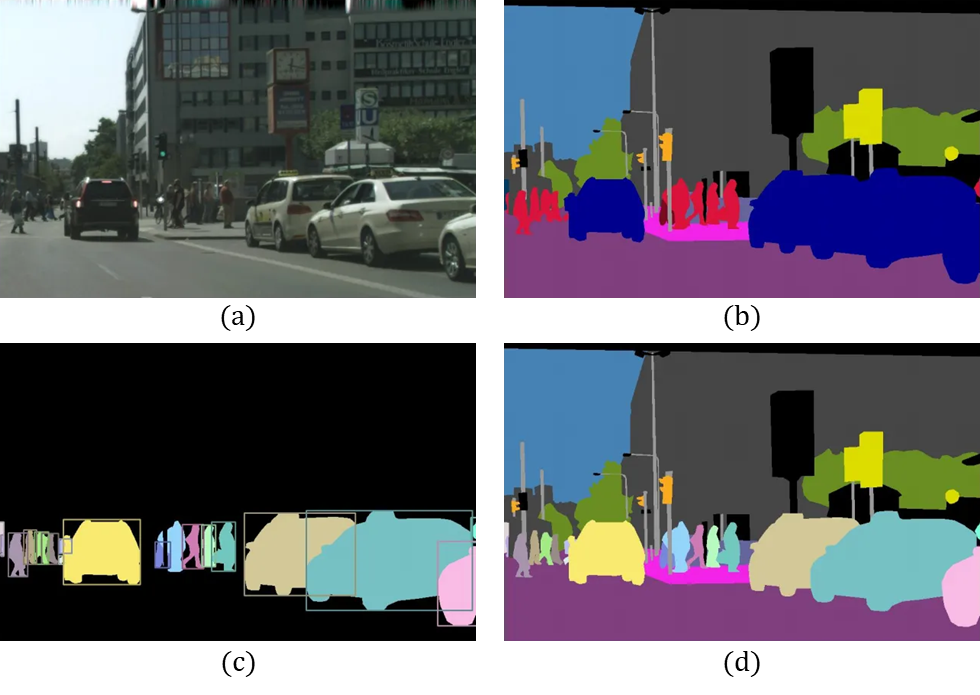
Semantic vs Instance vs Panoptic:

Note that, in semantic segmentation, there is no distinction between multiple instances of the same category, i.e., all Cars together are shown in blue and Persons in red, for example.
In instance segmentation, since the initial object detection step detects all the object instances present in the image, each ‘Thing’ — Car and Person — is segmented individually while all the ‘Stuff’ is ignored.
And in panoptic segmentation, there is a semantic segmentation of both ‘Things’ as well as ‘Stuff’ while each instance of a ‘Thing’ is also segmented individually.
And in panoptic segmentation, there is a semantic segmentation of both ‘Things’ as well as ‘Stuff’ while each instance of a ‘Thing’ is also segmented individually.
Conclusion:
The field of Computer Vision has several applications ranging from Autonomous Vehicle Driving to Medical Image Analysis, which employ these various Computer Vision tasks.
Since the first step to solving a problem is to define it well, I hope this article — demystifying various Computer Vision tasks — will be of good use to anyone breaking into the field of Computer Vision.
References:
[1] Kirillov et al., Panoptic Segmentation, 2019.
[2] He et al., Mask R-CNN, 2017.
[3] Redmon et al., You Only Look Once, 2015.
Your First Step Into The Field Of Computer Vision was originally published in Towards Data Science on Medium, where people are continuing the conversation by highlighting and responding to this story.
from Towards Data Science - Medium
https://towardsdatascience.com/your-first-step-into-the-field-of-computer-vision-f9928ecb313f?source=rss----7f60cf5620c9---4
via RiYo Analytics

No comments