https://ift.tt/QchjLrk An end-to-end machine learning solution for the Stellar Classification problem in Astronomy. Photo by Shot by Cerq...
An end-to-end machine learning solution for the Stellar Classification problem in Astronomy.

1. Introduction
Astronomy is the study of everything in the universe beyond Earth’s atmosphere. Astronomers use stellar classification to classify stars based on spectral characteristics. Spectral characteristics help astronomers extract more information about the stars — elements, temperature, density, and magnetic field.
The classification scheme of galaxies, quasars, and stars is one of the most fundamental in astronomy. This problem aims to classify stars, galaxies, and quasars (luminous supermassive black holes) based on spectral characteristics.
2. Dataset Overview
The data consists of 100,000 observations of space taken by the SDSS (Sloan Digital Sky Survey). Every data point is described by 17 feature columns and 1 class column which identifies it to be either a star, galaxy, or quasar [1].
Note: The SDSS data is under the public domain. Please refer to the citation at the end.
2.1. Features in the dataset
- obj_ID = Object Identifier, the unique value that identifies the object in the image catalog used by the CAS.
- alpha = Right Ascension angle (at J2000 epoch).
- delta = Declination angle (at J2000 epoch).
- u = Ultraviolet filter in the photometric system.
- g = Green filter in the photometric system.
- r = Red filter in the photometric system.
- i = Near Infrared filter in the photometric system.
- z = Infrared filter in the photometric system.
- run_ID = Run Number used to identify the specific scan.
- rereun_ID = Rerun Number to specify how the image was processed.
- cam_col = Camera column to identify the scanline within the run.
- field_ID = Field number to identify each field.
- spec_obj_ID = Unique ID used for optical spectroscopic objects (this means that 2 different observations with the same spec_obj_ID must share the output class).
- class = Object class (galaxy, star, or quasar object).
- redshift = Redshift value based on the increase in wavelength.
- plate = Plate ID, identifies each plate in SDSS.
- MJD = Modified Julian Date, used to indicate when a given piece of SDSS data was taken.
- fiber_ID = Fiber ID that identifies the fiber that pointed the light at the focal plane in each observation.
2.2. Background information useful to understand the data
2.2.1. Celestial sphere: The celestial sphere is an imaginary sphere that has a large radius and is concentric on Earth. All objects in the sky can be conceived as being projected upon the inner surface of the celestial sphere, which may be centered on Earth or the observer [2].
2.2.2. Celestial equator: The celestial equator is the great circle of the imaginary celestial sphere on the same plane as the equator of Earth [3].
2.2.3. Ascension and declination: Ascension and declination both are used in astronomy and navigation in space. Ascension tells how far left or right the object is in the celestial sphere and declination tells how far up or down the object is in the celestial sphere [4].
2.2.4. Photometric system: The word photo means light and metry means measurement. So, measuring the brightness of the light which a human eye can perceive is called photometry. The UBV photometric system (from Ultraviolet, Blue, and Visual), also called the Johnson system, is a photometric system usually employed for classifying stars according to their colors. It was the first standardized photometric system [5, 6].
2.2.5. Redshift: Redshift is a key concept for astronomers. The term can be understood literally — the wavelength of the light is stretched, so the light is seen as ‘shifted’ towards the red part of the spectrum. It reveals how an object in space (star/planet/galaxy) is moving compared to us. It lets astronomers measure the distance for the most distant (and therefore oldest) objects in our universe [7].
I understand that some features in the dataset are significantly useful such as navigation angles — ascension and declination, filters of the photometric system — u, g, r, i, z, and redshift. And, the rest of the other columns in the dataset are IDs that are not useful in the learning stage.
3. Machine Learning Problem Formulation
3.1. Type of machine learning problem
This is a multi-class classification problem as this dataset has 3 different target classes which need to be predicted.
3.2. Performance metrics that will be used to assess the model
3.2.1. Multi-class logloss: Logloss quantifies how close the prediction probability is to the corresponding actual/true value (in binary setup). Logloss extended for multi-class setup is called multi-class logloss.
3.2.2. Confusion matrix: It summarizes the confusion encountered by the learning model. The number of correct and incorrect predictions is shown with count values and broken down by each class.
4. Exploratory Data Analysis
4.1. Schema of the dataset
I read the dataset using pandas as a reference variable.
The below schema of the dataset shows that the dataset has no empty cells, and it also shows the datatype of each feature.
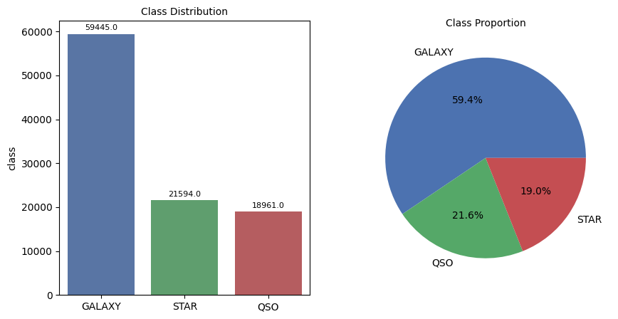
4.2. Distribution of the dataset
The below charts show the class distribution and class proportion in the data.
4.3. Univariate analysis
The univariate analysis takes individual features to analyze the data.
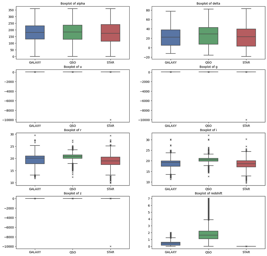
4.3.1. Boxplot
The boxplot is a visual representation of quartiles in a set of data. The below chart shows a boxplot of each feature based on the target class.
Another added advantage of using a boxplot is that I can quickly hunt for outliers. I can see that features — r, g, and z have one outlier value from the STAR class.
The boxplot of the redshift feature for the STAR class shows a 0 value, which means, for the model to categorize a data point as the STAR class with maximum accuracy should have a redshift of 0.
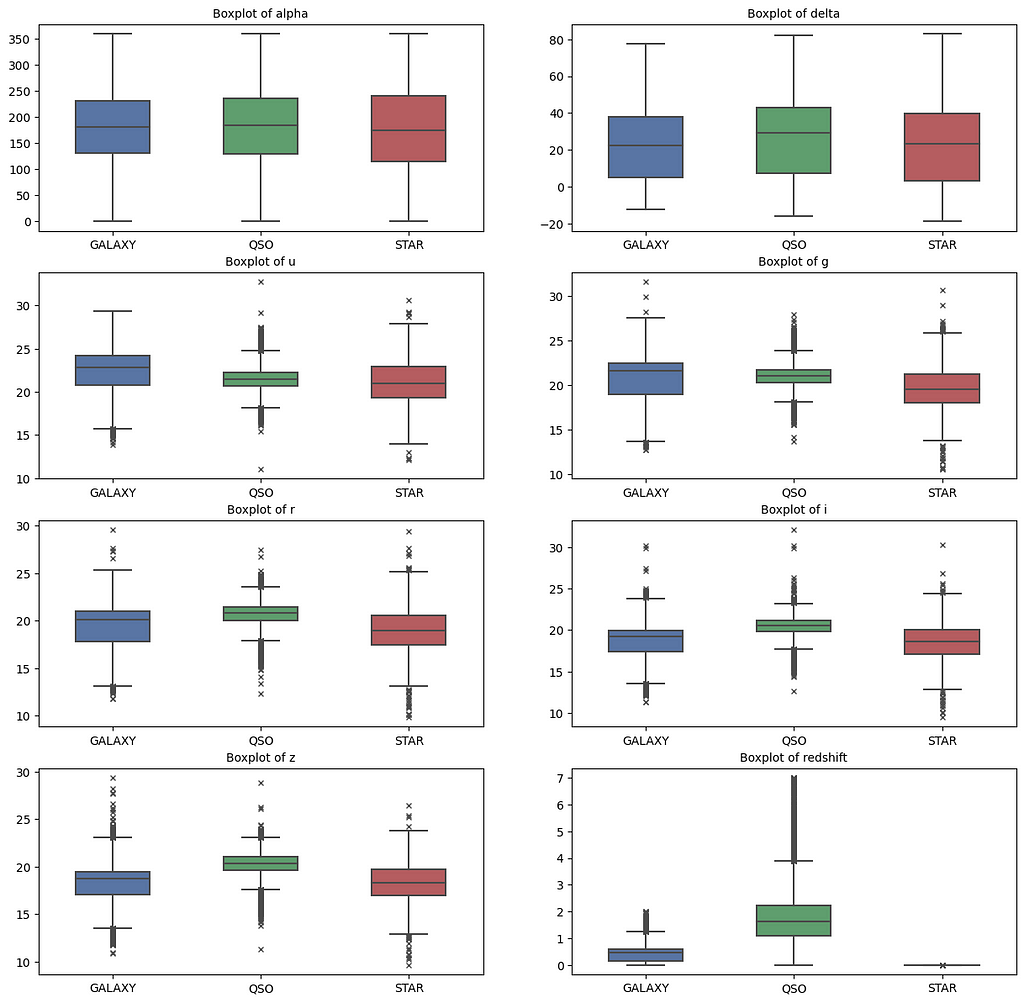
The below chart is the same boxplot, but after removing the outlier value from the dataset.
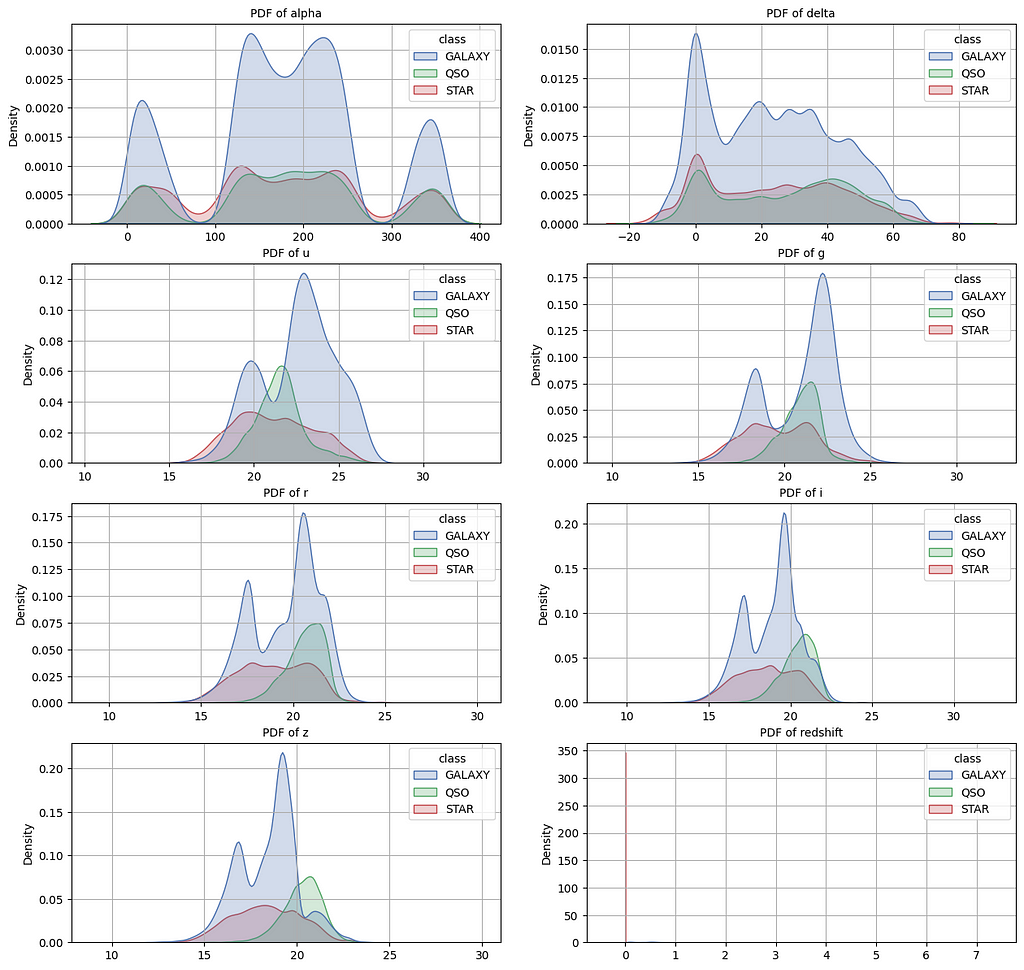
4.3.2 Density plot
The density plot is a visual representation of the PDF for a set of points. The PDF mainly shows the distribution of the data. The below chart shows a density plot of each feature based on the target class.
The classes in each density plot for a given feature are overlapping, which means, I cannot categorize the data by using simple logical statements. I have to employ a statistical model to categorize the classes of the data.
The density plot of the redshift feature for the STAR class conforms with the above boxplot.
4.4. Multivariate analysis
The multivariate analysis considers multiple features to analyze the data.
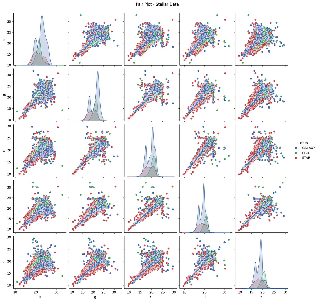
4.4.1 Pairplot
The pairplot visualizes the pairwise relationships in the data. The below pairplot illustrates the pairwise relationships of u, g, r, i, and z features. The conclusion is all the features (u, g, r, i, and z) are positively correlated with each other.
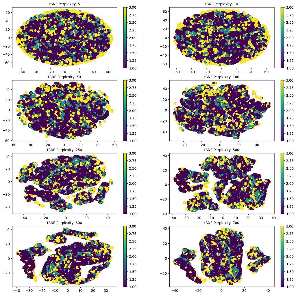
4.4.2. t-SNE plot
The t-distributed Stochastic Neighbor Embedding (t-SNE) is a tool to visualize high-dimensional data. It is a dimensionality reduction technique, but the new columns that it creates are not used for modeling as it does not produce a predictive model such that unseen data can be mapped to lower dimensions.
The below t-SNE plots for different perplexity values are an endeavor to better understand visually whether the data can be categorized on a lower dimension. The execution time to generate these plots took a couple of hours.
5. Feature engineering and feature importance
I will split the dataset into 3 sets — Train, Cross-validation, and Test sets. This is a good practice to test the model’s performance before deploying it in production.
- The train set will have 60% of the data.
- The cross-validation set will have 20% of the data.
- The test set will have 20% of the data.
As the dataset currently is imbalanced, I need to split the dataset by applying stratified sampling which keeps the diversity of the target variable intact.
Feature engineering should be implemented first on the train set followed by cross-validation and test sets to avoid data leakage.
5.1. Data normalization
The density plots of the features do not follow Gaussian distribution and the features are not having a consistent scale. It is important to bring the values of all the features into a consistent scale without distorting the meaning of the values.
5.2. Feature engineering
Feature engineering is the process of using domain knowledge to extract features from raw data via data mining techniques. These features can be used to improve the performance of machine learning algorithms. Feature engineering can be considered as applied machine learning itself [8].
5.2.1. Constructing new features by applying numerical operations
After many trials and errors, I constructed new features by subtracting r with g, u, i, and z and by subtracting z with i.
Total features now — u, g, r, redshift, g-r, i-z, u-r, i-r, z-r.
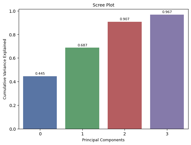
5.2.2. Principal component analysis (PCA)
PCA is a dimensionality reduction technique. It detects linear combinations of the input features that can best capture the variance in the entire set of features, where the components are orthogonal to and not correlated with each other.
Using the scikit-learn library, I set the components to 0.95 (meaning PCA will find out new components that will preserve 95% of the variance in the entire dataset). The PCA identified 4 components that preserve 95% variance.
5.2.3. Testing the feature-engineered features and PCA components on logistic regression
I built 3 logistic regression models.
- Model 1 for only feature-engineered features.
- Model 2 for only PCA components.
- Model 3 for feature-engineered features and PCA components.
Model 2 (only PCA components) performed poorly. The performance of Model 3 (feature-engineering + PCA) and Model 1 (only feature-engineering) is similar which means PCA components are not adding much useful information in addition to already feature-engineered features.
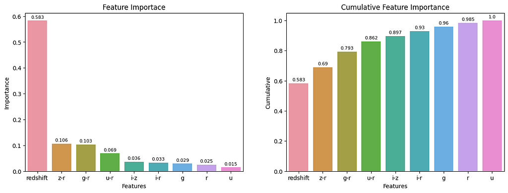
5.3. Feature importance
Feature importance is the process of identifying important features from which the model can learn effectively. This technique aims to score the features, so I can pick the features whose score is high.
I developed a Random Forest model to get the essential features. The below feature importance plot clearly illustrates that features — r, and u are the least important.
6. Modeling
6.1. Hyperparameter tuning
Hyperparameters control the learning process of the model. In this process, the learning model is exposed to a set of values for each parameter and then the best parameter value is selected. This process is called tuning. The performance metric for tuning is typically measured by cross-validation on the training set.
I used RandomizedSearchCV for tuning the hyperparameters.
I used a series of classification and ensemble algorithms in this stage. The aim is to try as many models as possible. I will not put all the code here because the blog will become large, but the code is on my GitHub profile.
Code link for modeling: here.
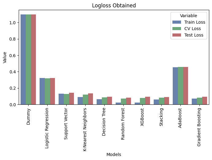
The ensemble models namely, the Random Forest classifier and XGBoost classifier seem to have signs of overfitting as training loss is significantly less than cross-validation and test losses.
However, the Stacking Classifier performed better and is not showing signs of overfitting. In this classifier, I stacked Logistic Regression, Support Vector Classifier, K Neighbors Classifier, and Decision Tree Classifier with their best parameters.
6.2. Stacking classifier model
A stacking classifier is an ensemble technique that combines multiple learning models (learners) to form a powerful model. The final prediction is obtained by combining the predictions of each learner.
6.2.1. Code
In the below snippets, I used some custom functions I defined in the notebook, you can please refer to them from the above link.
6.2.2. Output
In the next sub-section, I will present you with the performance summary report of all the models trained to solve the stellar classification problem.
6.2. Summary of all the models applied
+----+---------------------+--------------+-----------+-------------+
|    | Models              |   Train Loss |   CV Loss |   Test Loss |
|----+---------------------+--------------+-----------+-------------|
|  0 | Dummy               |        1.099 |     1.099 |       1.099 |
|  1 | Logistic Regression |        0.322 |     0.319 |       0.324 |
|  2 | Support Vector      |        0.133 |     0.13  |       0.143 |
|  3 | K-Nearest Neighbors |        0.091 |     0.12  |       0.137 |
|  4 | Decision Tree       |        0.065 |     0.086 |       0.094 |
|  5 | Random Forest       |        0.024 |     0.072 |       0.084 |
|  6 | XGBoost             |        0.022 |     0.08  |       0.093 |
|  7 | Stacking            |        0.061 |     0.082 |       0.09  |
|  8 | AdaBoost            |        0.456 |     0.457 |       0.459 |
|  9 | Gradient Boosting   |        0.073 |     0.082 |       0.093 |
+----+---------------------+--------------+-----------+-------------+
7. Productionization of ML Application
Productionization is the process to expose the machine learning model to the outside world from the Jupyter Notebook environment.
7.1. Deploying the model on a local application
In this sub-stage, I exported the Stacking Classifier object along with the feature-scaling object to disk. I then created a frontend interface with help of Dash.
7.1.1. Local application demo
7.2. Deploying the local application to the cloud
I had to rework on frontend interface from the Dash interface to the Streamlit interface. AWS Elastic Beanstalk was not allowing my Dash application, and the health of the Elastic Beanstalk environment was either degraded/severe (I guess some configuration issue on my end).
I finally decided to go with the Streamlit interface. In Streamlit, deploying any data science or machine learning application is quick and easy.
7.2.1. Cloud application URL
URL: https://mohd-saifuddin-stellar-classification-app-app-izkfa9.streamlit.app/
8. Learning Outcomes
My learning outcomes working on this project.
- I learned how to approach a research problem as a machine learning problem.
- I learned to perform detailed EDA — univariate analysis and multivariate analysis.
- I learned to perform data processing.
- I learned feature engineering and feature importance. In this process, having domain knowledge or consulting an expert in the field yields fruitful results.
- I learned modeling with different algorithms.
- Finally, I learned the productionization of machine learning models to the frontend application.
9. References
[1] Abdurro’uf et al., The Seventeenth data release of the Sloan Digital Sky Surveys: Complete Release of MaNGA, MaStar and APOGEE-2 DATA (Abdurro’uf et al. submitted to ApJS) [arXiv:2112.02026].
[2] Celestial sphere. (2022, November 21). Wikipedia. here.
[3] Celestial equator. (2021, October 30). Wikipedia. here.
[4] Galactic Sphere, Declination, Right Ascension. (2017, June 17). YouTube. here.
[5] UBV photometric system. (2022, October 13). Wikipedia. here.
[6] Photometric system. (2022, November 18). Wikipedia. here.
[7] What is ‘red shift’? European Space Agency. here.
[8] Feature engineering. (2022, November 2). Wikipedia. here.
10. End
Thank you for reading. If you have any suggestions, please let me know.
You can connect with me on LinkedIn: here.
Stellar Classification: A Machine Learning Approach was originally published in Towards Data Science on Medium, where people are continuing the conversation by highlighting and responding to this story.
from Towards Data Science - Medium
https://towardsdatascience.com/stellar-classification-a-machine-learning-approach-5e23eb5cadb1?source=rss----7f60cf5620c9---4
via RiYo Analytics


No comments