https://ift.tt/j1BqaX3 Clear and Visual Explanation of the K-Means Algorithm Applied to Image Compression with GIFs How K-Means can be use...
Clear and Visual Explanation of the K-Means Algorithm Applied to Image Compression with GIFs
How K-Means can be used to significantly reduce the file size of an image.
In this guide, I describe and implement the k-means algorithm from scratch and apply it to image compression. I use different visualizations to help the reader develop a stronger understanding of the k-means algorithm and how it can be used for image compression. I also discuss various advantages and limitations of this approach towards the end.
All images unless otherwise noted are by the author, available here.
What is the K-Means Algorithm?
The k-means algorithm is an unsupervised algorithm that partitions a dataset into k distinct clusters. It is unsupervised, meaning there are no labels for the data points. In other words, we don’t have prior knowledge of how the dataset should be clustered. We simply provide the dataset as is, and use k-means to partition it into k clusters.
Big Picture Idea
K-means seeks to divide a dataset into k clusters where members of each cluster share characteristics and are different from other clusters. Therefore, the goal is for k-means to divide the dataset meaningfully into k different clusters.
Applications
Cluster analysis groups similar data together by abstracting the underlying structure of a dataset, which can provide meaningful insight. “Clustering has been effectively applied in a variety of engineering and scientific disciplines such as psychology, biology, medicine, computer vision, communications, and remote sensing” [1].
How the K-Means Algorithm Works
The K-means algorithm is broken into several steps:
- Initializing a set of cluster centroids
- Assigning observations to clusters
- Updating the clusters
Steps 2 and 3 are repeated for either a set number of iterations or until convergence, which occurs when the cluster centroids no longer change.
Let us dive deeper into each of these steps.
1. Initializing the set of cluster centroids
The first step to initializing the set of cluster centroids is choosing how many centroids we want to use, which we refer to as k.
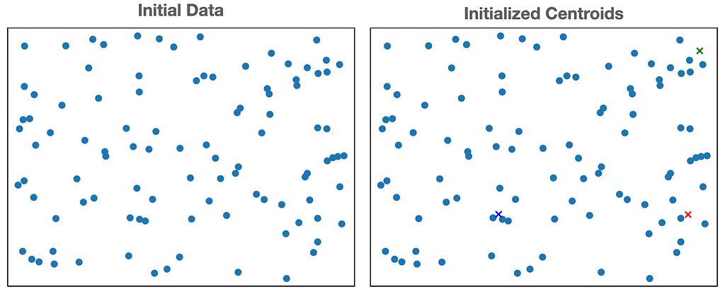
Once, we have chosen the number of clusters, we choose k samples randomly from the training examples, and set the cluster centroids to be equal to the values of the selected k examples. Alternatively, we can randomly sample k different points in the solution space to initialize the cluster centroids.
We refer to the j-th centroid as μⱼ, because it represents the mean of the values assigned to cluster j. This is where the name k-means arises from. In the figure below, we set k=3 and randomly sample 3 points in the sample space (represented by green, blue, and red ‘x’) to initialize the cluster centroids.
2. Assigning Observations to Clusters
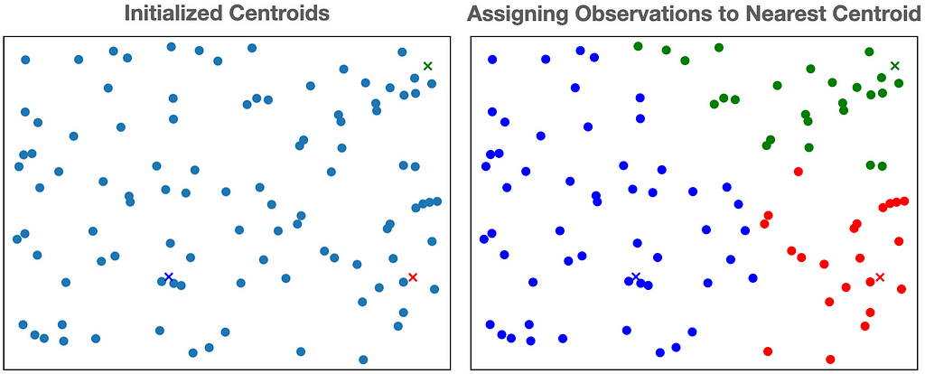
Now that we have our k centroids, we assign each observation (data point) to the centroid closest to it. Typically, we calculate “closeness” using the euclidean distance. In the figure below, we illustrate the process of assigning the observations to the 3 centroids above.
3. Updating the Centroids
Once all of the observations have been assigned to a cluster, we shift the centroid of each cluster to the mean of its assigned observations. We illustrate this process below.
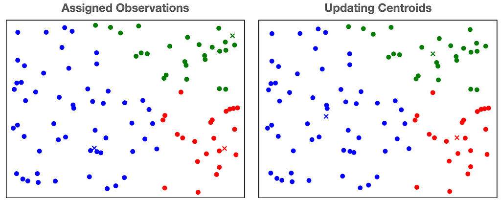
Repeat till convergence or for a certain number of iterations
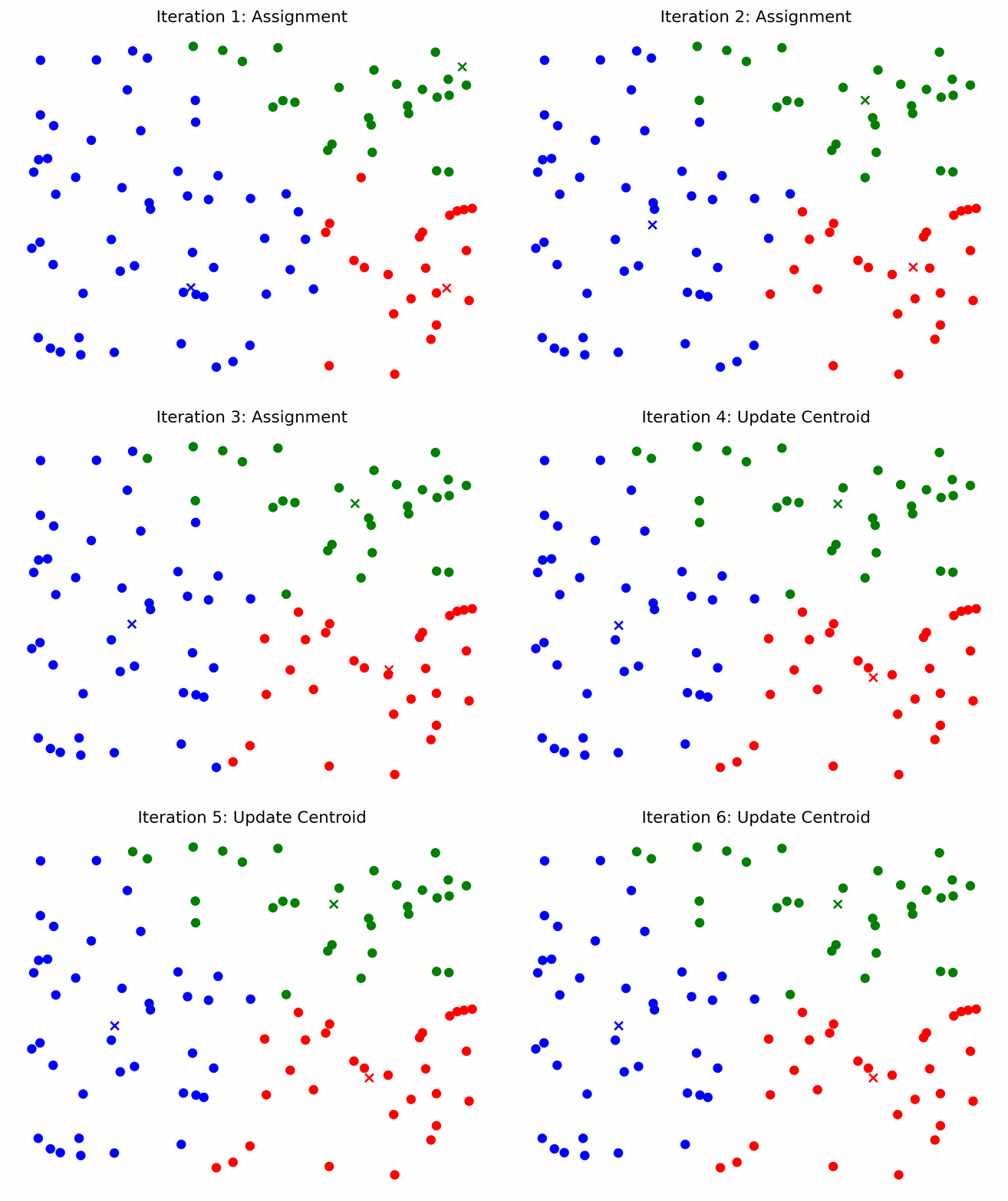
Each iteration of the k-means algorithm consists of two parts: Step 2 (Assigning Observations to Clusters) and Step 3 (Updating the Clusters). This process is repeated for either a set number of iterations or until convergence. Convergence occurs when the cluster centroids no longer change. This is equivalent to saying that the assignments of the observations do not change anymore.
The k means algorithm will always converge within a finite number of iterations [2] but it is susceptible to local minima [3].
In the example below, the k means algorithm converges at iteration 4. This is because the cluster centroids no longer change after iteration 4.
K-Means for Image Compression
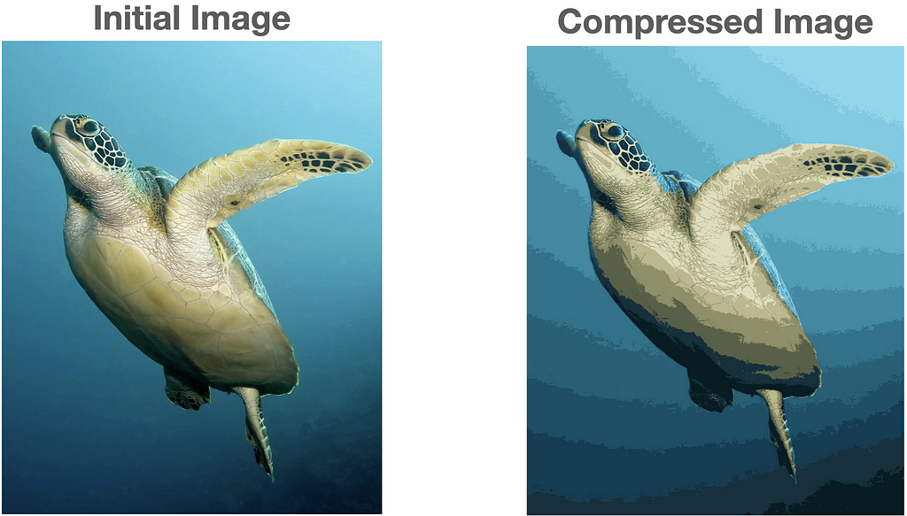
The goal of image compression is to reduce the file size of an image. We can use K-means to select k colors to represent an entire image. This allows us to represent an image using only k colors, instead of the entire RGB space. This process is also referred to as image quantization.
Why K-means is useful for image compression
The purpose of using k-means for image compression is to select k colors to represent a target image with the least approximation error. In other words, we will be using k-means to find the best k colors to represent a target image with.
How K-means provides compression
The color pixels in an image are represented by their RGB values, which each range from 0 to 255. Since each color band has 256=2⁸ settings, there are a total of 256 ⋅ 256 ⋅ 256 = 256³ = 2²⁴ ~ 17 million colors. To represent each of these colors for any pixel, computers need log₂(2²⁴) = 24 bits of storage space. If we use K-means to select 16 colors that we represent an entire image with, we only need log₂(16) = 4 bits. Therefore, by using K-means with k=16, we can compress the image size by a factor of 6!
Now that we understand the theory, let us dive into some code and visualizations.

Reading in the Image and Initializing the Centroids
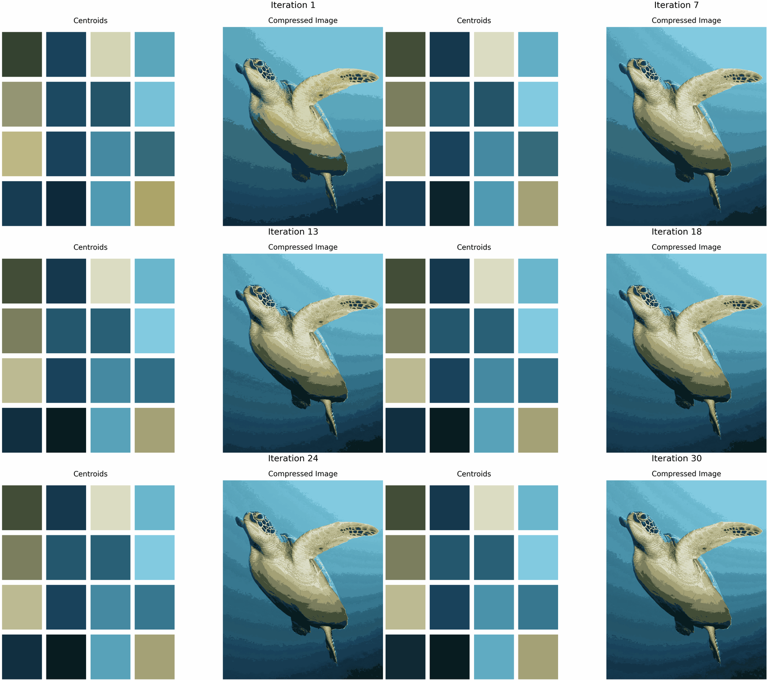
In the context of image compression, the centroids are the colors we are using to represent the compressed image. Therefore, our first step is to read in the image and select k random colors from the image to initialize our centroids.
In line 7, we read in the image using numpy. This produces a 2 dimensional array where each element is a list of length 3 that represents the RGB values of that pixel. Remember to modify image_path to your own.
Starting on line 9, we define the function to initialize our centroids. We select a random pixel from the image and add its corresponding RGB value to the centroids_init array. We do this k = num_clusters times. Thus, centroids_init is an array of k colors sampled randomly from our image.
Assigning and Updating Centroids
To iteratively update our centroids, we repeat the process of assigning observations to cluster centroids and updating the centroids to be the mean of the assigned observations.
In the context of image compression, this means assigning each pixel of the target image to the centroid color that is nearest to it.
In lines 11–17, we are creating the dictionary centroid_rgbs . Each key corresponds to an index of the centroids and the values are a single numpy array that contain all of the colors assigned to the corresponding centroid.
The assignment of each pixel to a centroid is done on line 13 using linalg.normto calculate the euclidean distance to each centroid and then using argminto find the index of the nearest centroid.
Creating the Compressed Image
Now that we have the finalized centroids, we can create the compressed image. We simply iterate through each pixel and change its color to the nearest centroid.
Putting Everything Together
With the following snippet and the function definitions above, all the pieces to running k-means for image compression are complete.
To generate the GIF’s, I used plt.savefig at various stages of the algorithm. My github repository contains the code for that process, and how to convert those frames to a GIF [4].
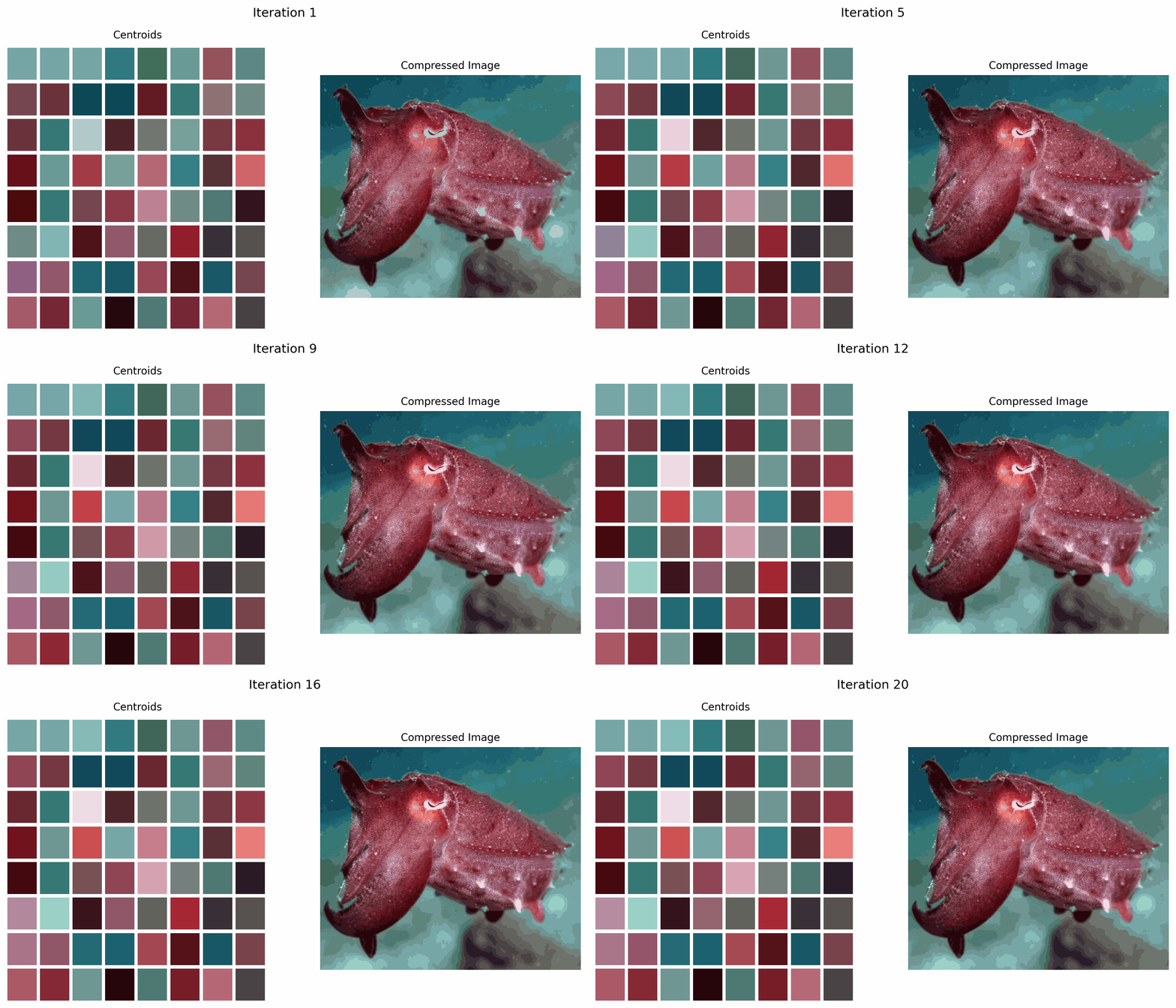
In the GIF above, we see how the centroids, which are the colors we choose to represent the image, change over time as the k-means algorithm iterates.
Analysis of K-Means for Image Compression
Now, we analyze some details regarding the use of k-means for image compression.
Outliers
Often, images will contain outlier colors relative to the main color palette of the image. For example, the target image below contains two small clown-fish that are bright orange. Their color contrasts strongly from the dark background and sea anemone, which draws the viewers attention to them (hopefully in an aesthetically pleasing way).
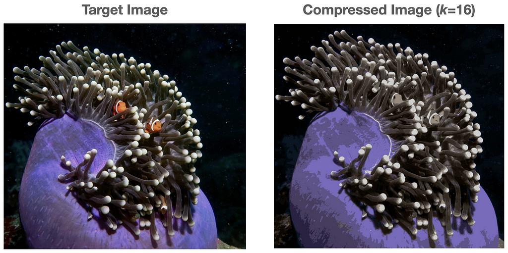
The GIF below illustrates what happens when we apply k-means to this image for k=16. Although the clown-fish’s bright orange is selected as an initial cluster, it is eventually ‘washed out’ by the darker colors as the algorithm iterates.
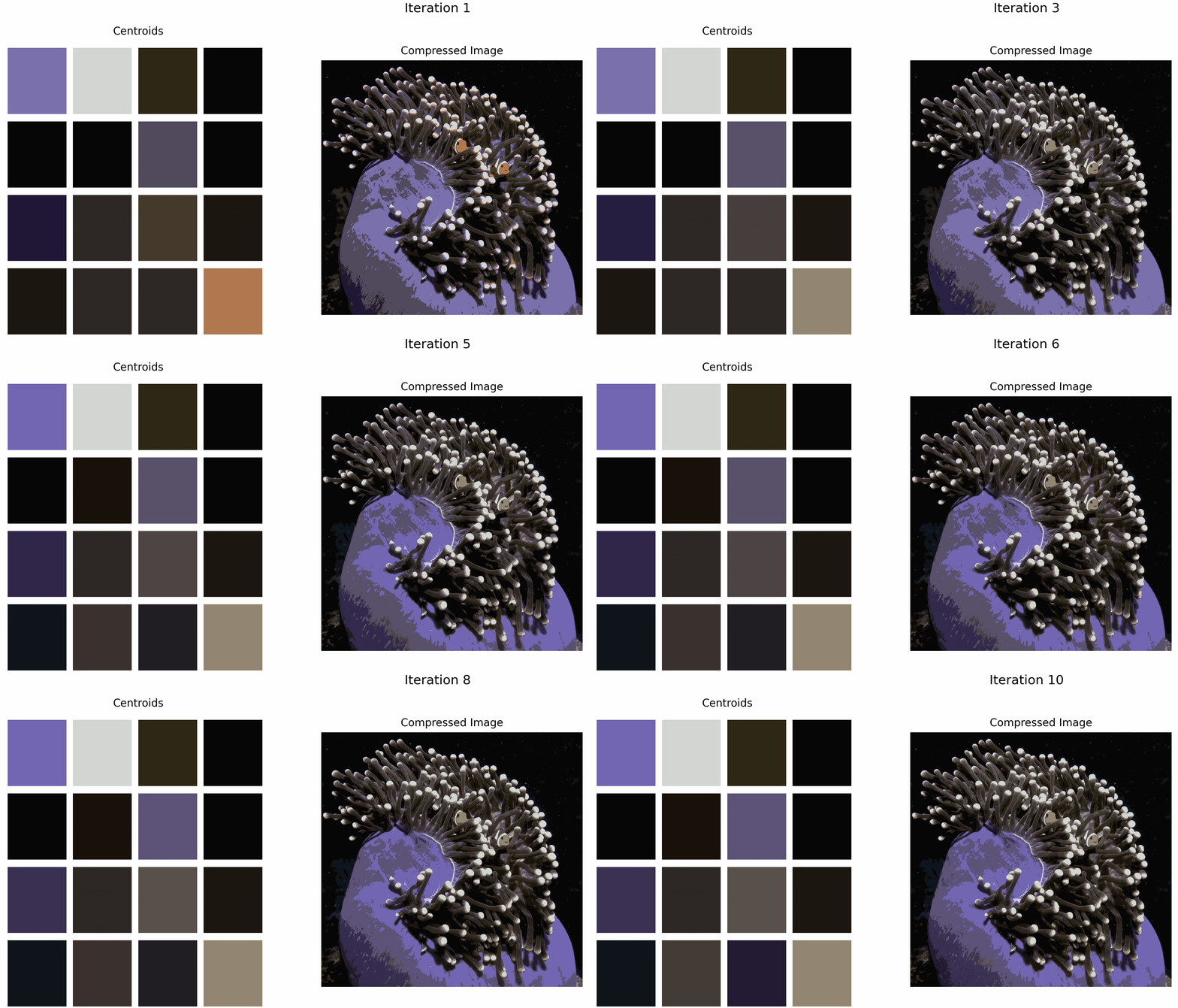
Although the overall quality of the compressed image increases as the number of iterations increases, the accuracy of the outlier color decreases.
Some literature suggests creating clusters specifically for outliers (calculated using a distance metric) to improve overall clustering accuracy [5]. The authors’ use of numerical experiments on both synthetic data and real data are provided to demonstrate the effectiveness and efficiency of their proposed algorithm. I suspect that implementing this algorithm could help with image compression using k-means, especially with images that contain outlier colors.
Selecting “k”
The choice of k determines the amount of compression, and is up to the user to set. A higher value of k will provide for a more faithful representation of the target image, but comes at the cost of lower compression. In the graphic below, we illustrate compressed images with increasing values of k. The compression factors for k=16, k=32, k=64, and k=128 are 6, 4.8, 4, and 3.4 respectively.
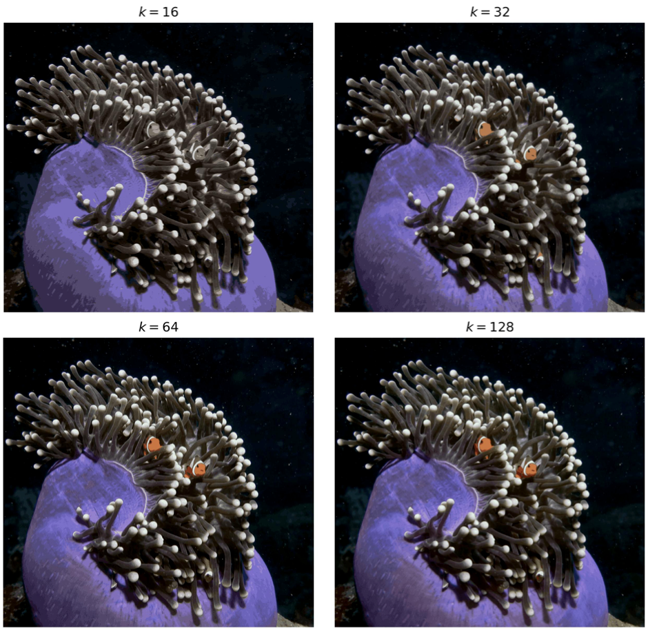
In the example above, we see that choosing a k value greater than 32 is critical in mitigating the outlier issue mentioned in the previous section. Since k is large enough, at least one centroid is able to be assigned to the bright orange color. In the figure below, we plot the centroid colors after 30 iterations for both k=64 and k=256.
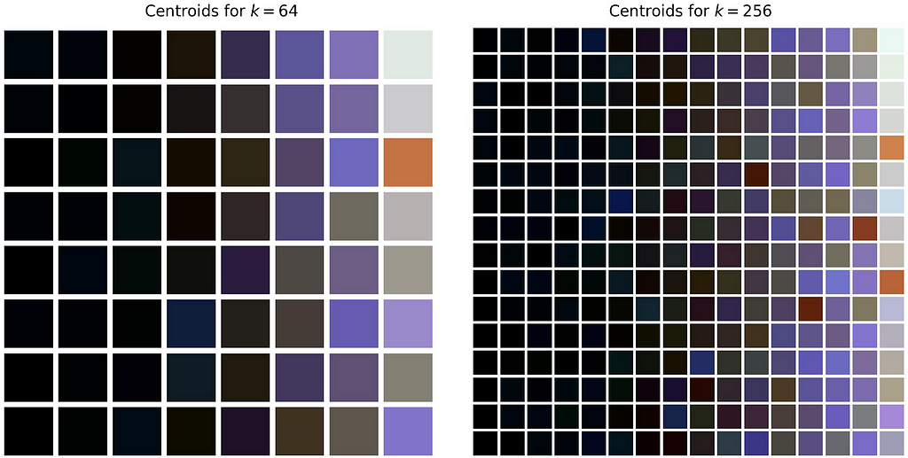
After 30 iterations, k=64 has one centroid that is assigned to orange. For k=256, there are approximately 4 shades of orange.
This visualization also portrays the compression amount vs. detail trade-off for different k-values. Clearly for larger values of k, we have more colors and retention of detail, however we require more data to represent those colors.
It is likely worth experimenting with different values of k depending on the target image and use case.
Lossy Compression
Using the k-means algorithm to compress an image is a form of lossy compresion. Lossy compression is a class of data compression that uses approximations and partial data loss of a target image [6]. When we use k-means for image compression, we are approximating each pixel’s color using the nearest centroid. Since we are losing information in this process, we cannot revert the compressed image back to the original. This is why lossy compression is also refered to as irreversible compression.
On the other hand, lossless data compression does not lose information. Instead, it uses techniques to represent the original information using less data [7]. However, the amount of compression that is possible using lossless data compression is much lower than that of lossy compression.
Although k-means is a form of lossy compression, the loss of detail can be almost in-perceivable to the human eye for certain values of k.
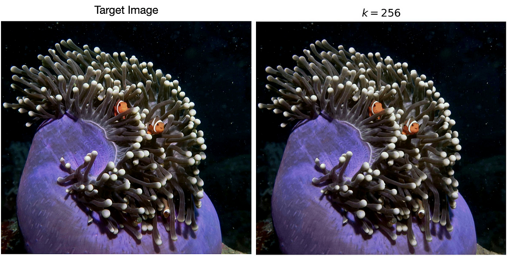
Can you notice many differences between the two images above? Using k=256, the compressed image on the right requires only 1/3 the amount of data compared to the full image on the right!
Randomness in Centroid Initialization
Holding everything in regards to k-means constant, each run will differ slightly as a result of the randomness inherent in the centroid initialization process.

This means that the compressed images given the same parameters will output slightly different variations. However, for larger values of k, this effect is not as apparent to the human eye.

Advantages and Disadvantages
Now that we have completed a thorough analysis of the k-means algorithm in regards to image compression, we will explicitly discuss its advantages and disadvantages.
Advantages
- Efficiency: The k-means algorithm is computationally efficient (linear time complexity), making it suitable for real-time image compression applications [8]. This also means it can handle large images.
- Simplicity: The k-means algorithm is relatively simple and easy to understand.
- Great for certain types of images: k-means performs well on images with distinct clusters of similar colors.
Disadvantages
- Lossy Compression Algorithm: K-means is a form of lossy compression that represents an entire image based on clusters of pixels, therefore it loses some color information and may not preserve fine details in an image.
- Sensitivity to initialization: The performance of the k-means algorithm can be sensitive to the initial positions of the centroids, which can lead to sub-optimal or inconsistent results. This is less of a problem with larger values of k.
- Not suitable for certain types of images: k-means algorithm perform poorly on images with smooth color gradients and images with high noise.
Conclusion
Overall, k-means can be a good choice for lossy image compression, especially for images with distinct clusters of similar colors. However, it may not be the best choice for all types of images and other techniques such as vector quantization or fractal compression may produce better results.
The user has a critical decision to make when selecting the value of k, and must keep in mind the ‘compression amount vs. detail trade-off’ discussed in the “Selecting ‘k’” section. The optimal k value will likely vary according to the user’s needs.
Hopefully the different visualizations were able to help develop a stronger understanding of the k-means algorithm, and how it can perform image compression.
References
[1] Krishna, K., and M. Narasimha Murty. “Genetic K-Means Algorithm.” IEEE Transactions on Systems, Man and Cybernetics, Part B (Cybernetics), vol. 29, no. 3, 1999, pp. 433–439., https://doi.org/10.1109/3477.764879.
[2] https://stats.stackexchange.com/questions/188087/proof-of-convergence-of-k-means
[3] Ng, Andrew. “CS229 Lecture Notes.” https://cs229.stanford.edu/notes2022fall/main_notes.pdf
[4] My Github Repository with the code for this project. https://github.com/SebastianCharmot/kmeans_image_compression
[5] Gan, Guojun, and Michael Kwok-Po Ng. “K -Means Clustering with Outlier Removal.” Pattern Recognition Letters, vol. 90, 2017, pp. 8–14., https://doi.org/10.1016/j.patrec.2017.03.008.
[6] “Lossy Compression (Article).” Khan Academy, Khan Academy, https://www.khanacademy.org/computing/computers-and-internet/xcae6f4a7ff015e7d:digital-information/xcae6f4a7ff015e7d:data-compression/a/lossy-compression.
[7] Ming Yang, and N. Bourbakis. “An Overview of Lossless Digital Image Compression Techniques.” 48th Midwest Symposium on Circuits and Systems, 2005., 2005, https://doi.org/10.1109/mwscas.2005.1594297.
[8] Chiou, Paul T., et al. “A Complexity Analysis of the JPEG Image Compression Algorithm.” 2017 9th Computer Science and Electronic Engineering (CEEC), 2017, https://doi.org/10.1109/ceec.2017.8101601.
Clear and Visual Explanation of the K-Means Algorithm Applied to Image Compression was originally published in Towards Data Science on Medium, where people are continuing the conversation by highlighting and responding to this story.
from Towards Data Science - Medium
https://towardsdatascience.com/clear-and-visual-explanation-of-the-k-means-algorithm-applied-to-image-compression-b7fdc547e410?source=rss----7f60cf5620c9---4
via RiYo Analytics

No comments