https://ift.tt/yXo5KHN What exactly is going on in AI systems plagued by biases? Photo by Pawel Czerwinski on Unsplash The problem of...
What exactly is going on in AI systems plagued by biases?

The problem of bias in artificial intelligence (AI) has made many negative headlines recently. The reports showed that AI systems have the potential to unintentionally discriminate against sensitive subgroups. For example, an AI-powered recruiting system by an international technology company was found to systematically favour male applicants over female ones. In this article, I will shed some light on the inner processes which take place when AI goes rogue. It is inspired by a research paper I published on the topic.[1]
In order to gain a better understanding of the background to this problem, let us first introduce some fundamental knowledge about machine learning. Compared with traditional programming, one major difference is that the reasoning behind the algorithm’s decision-making is not defined by hard-coded rules which were explicitly programmed by a human, but it is rather learned by example data: thousands, sometimes millions of parameters get optimised without human intervention to finally capture a generalised pattern of the data. The resulting model allows to make predictions on new, unseen data with high accuracy.
Example, please
To illustrate the concept, let’s consider a sample scenario about fraud detection in insurance claims. Verifying the legitimacy of an insurance claim is essential to prevent abuse. However, fraud investigations are labour intensive for the insurance company. In addition, for some types of insurance, many claims may occur at the same time — for example, due to natural disasters that affect entire regions. For policyholders, on the other hand, supplementary checks can be annoying, for example when they are asked to answer further questions or provide additional documents. Both parties are interested in a quick decision: the customers expect a timely remedy, and the company tries to keep the effort low. Therefore, an AI system that speeds up such a task could prove very useful. Concretely, it should be able to reliably identify legitimate insurance claims in order to make prompt payment possible. Potentially fraudulent cases should also be reliably detected and flagged for further investigation.
How is your AI performing?
Now, let’s dig into the technical bits. In order to assess the performance of such a classifier, we usually compare the predicted output Ŷ with the true output value Y. In the claims data, the output value 1 stands for a fraudulent claim, while 0 represents a legitimate claim. The following table contains sample predictions for our running example.

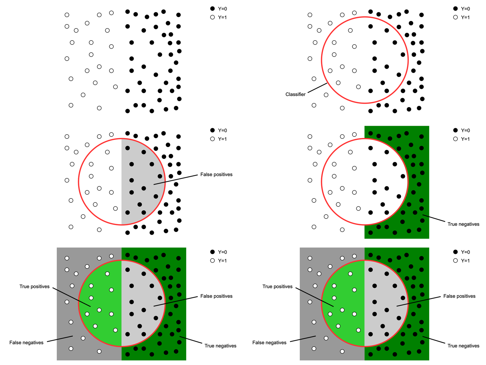
For better illustration, find the same results graphically represented in the animation below. The black dots correspond to the negative samples (Y=0), here actual legitimate claims. The white dots represent positive samples (Y=1), actual fraudulent claims in the present scenario. The big red circle constitutes the boundary of the classifier: Dots outside the circle have been predicted as negative/legitimate (Ŷ=0), dots inside the circle as positive/fraudulent (Ŷ=1). The different background colours further show where the classifier was right (light green and dark green), and where not (light grey and dark grey).
It is worth noting that in this oversimplified 2-dimensional example, drawing an ideal border which separates black and white dots and thus defining a perfect classifier would be obvious. In high-dimensional real world use cases, however, it is hardly possible to obtain a perfect classifier with error rates of zero; optimisation always remains a matter of trade-offs.

End the confusion
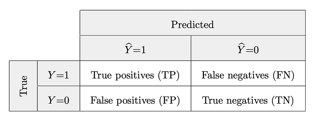
A so-called “confusion matrix” helps to visualise and compute statistical measures commonly used to inspect the performance of a ML model. The rows of the matrix represent the actual output classes, in our case 0 or 1. The columns represent the predicted output classes by the given classifier. The cells where the predicted class corresponds to the actual class contain the counts of the correctly classified instances. Wherever the classes differ, the classifier got it wrong and the numbers represent incorrectly classified samples.
On an abstract level, the figures in the cells are generally identified by the terms provided in the table below.

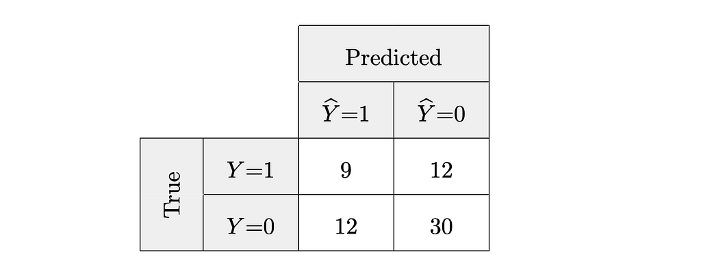
Taking the data from our running example as a basis, the related confusion matrix looks as follows. As you have noticed, the given classifier correctly predicted 9 claims to be fraudulent and 30 claims to be legitimate. However, it also falsely predicted 12 claims to be legitimate, which were in fact fraudulent, and 12 claims to be fraudulent, which really were not.

Revisiting the animated illustration above, we further realise that the coloured segments in the schema correspond to the different cells in the confusion matrix: true positives (light green), false positives (light grey), true negatives (dark green), and false negatives (dark grey).
Bring on the formulas!
From the confusion matrix we can extract plenty of interesting statistical measures. First, we count the actual positives in the data set. This number is the sum of the true positives and the false negatives, which can be viewed as missed true positives. Likewise, the number of actual negatives is the sum of the true negatives and the false positives, which again can be viewed as missed true negatives. In our example, those figures represent the numbers of actual fraudulent claims and actual legitimate claims.

The (positive) base rate, sometimes also called the prevalence rate, represents the proportion of actual positives with respect to the entire data set. In our example, this rate describes the share of actual fraudulent claims in the data set.

The true positive rate and the true negative rate describe the proportions of correctly classified positive and negative instances, respectively, of their actual occurrences. In the example, the true positive rate describes the share of all actual fraudulent claims which were detected as such. The true negative rate is the share of actual legitimate claims which were successfully discovered.

The false discovery rate describes the share of misclassified positive classifications of all positive predictions. So, it is about the proportion of positively classified instances which were falsely identified or discovered as such. On the contrary, the false omission rate describes the proportion of false negative predictions of all negative predictions. These instances, which are actually positive, were overlooked — they were mistakenly passed over or omitted. In our example, the false discovery rate is the error rate of all claims which were classified as fraudulent. The false omission rate describes the share of actually fraudulent claims of all claims which were classified as legitimate.

Plenty of other statistical measures exist to assess the performance of a ML model. However, for the purpose of demonstrating AI bias, the metrics introduced above are sufficient.
You overlooked something
Up until here, we have analysed the data as one population and did not consider the possible existence of sensitive subgroups in the data. However, since decisions from ML algorithms often affect humans, many data sets contain sensitive subgroups by nature of the data. Such subgroups may for example be defined by gender, race or religion. To analyse if a classifier is potentially biased, we add this extra dimension and split the results by this sensitive attribute into subgroups. This allows for investigation of possible discrepancies among them. Any such deviation could be an indicator for discrimination against one sensitive group.
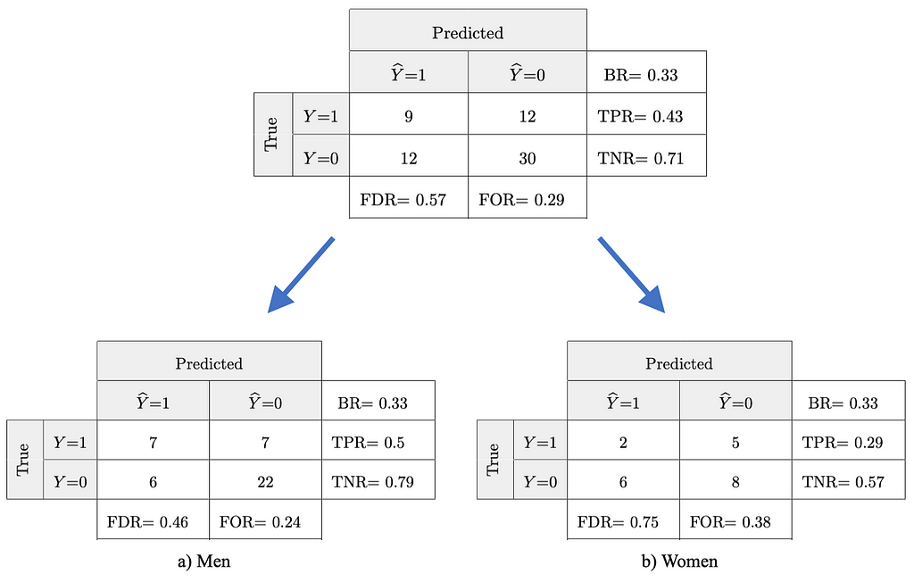
We now examine our running example on insurance fraud detection for unwanted bias. The output from the trained model remains unchanged, but this time we assume two sensitive subgroups in the data, for instance we split the data into men and women.

We notice that the base rates (BR) are identical in both subgroups which means in this example that men and women are equally likely to file a fraudulent (or a legitimate) claim. However, the true negative rate (TNR) for men is 0.79, while for women it is 0.57. This means 79% of the valid claims filed by men get correctly classified as legitimate, while for women that’s the case for only 57% of the same type of claims. On the other hand, the false omission rate for men is 24% and for women it is 38%. So, fraudulent claims filed by women have a higher chance to remain undetected than fraudulent claims filed by men in our fictional sample scenario.
So what
AI bias is said to occur when statistical measures, such as the ones described above, significantly differ from one sensitive subgroup to another. In other words, the system is biased when it performs differently for different groups. Due to the black box nature of most machine learning algorithms, and in particular in application areas where the output cannot be directly evaluated by the human eye (e.g. scores), this problem can remain unnoticed for a long time. Since AI has an ever-increasing impact on people’s lives, however, it is mandatory to detect and mitigate AI bias in order to prevent systematic unequal treatment of individuals from sensitive subgroups and instead ensure the responsible use of AI.
Now that we have a clearer idea of what exactly is going wrong in biased AI, we can turn our attention to the source of the problem. In my next article, I deepen the question where these biases actually come from.
Many thanks to Antoine Pietri for his valuable support in writing this post. All images unless otherwise noted are by the author.
References
[1] B. Ruf and M. Detyniecki, Towards the Right Kind of Fairness in AI (2021), ECML/PKDD Industry Track.
Biased AI, a Look Under the Hood was originally published in Towards Data Science on Medium, where people are continuing the conversation by highlighting and responding to this story.
from Towards Data Science - Medium
https://towardsdatascience.com/biased-ai-a-look-under-the-hood-5d0a41968f16?source=rss----7f60cf5620c9---4
via RiYo Analytics

No comments