https://ift.tt/loKXbvn From clustering to algorithm: a journey in five steps Image by Pauline Allouin While this article is more techni...
From clustering to algorithm: a journey in five steps
While this article is more technical than my previous ones – one of which was how to successfully translate tech talk for management and users — it aims to explain a popular algorithm used in data science in simple words. Recently, I had to explain what clustering is to a curious, non-technical senior manager. He understood the whole concept of clustering and wanted to know more about how it was translated into an algorithm.
The explanations in this post go way beyond the simple senior manager explanation, but I thought I would share that interesting experience; here I attempt to provide more details that we can usually find with an online search. Thus, it might provide answers to questions people have when implementing the K-means algorithm for the very first time. Also, I do not intend to repeat the many resources available on the internet but rather focus on its essence. At the end of each paragraph I will highlight the point that could be communicated to a less technical audience.
The big picture
Clustering is a technique for dividing a set of data points into groups (or clusters) based on their similarities. This method has many applications such as behavioural segmentation, inventory categorization, identifying groups in health monitoring, grouping images, detecting anomalies, etc. It can be used to explore or expand knowledge of a specific domain, especially when the datasets are too large to be analysed with traditional tools.
A commonly used example is customer segmentation: based on different factors (age, gender, income, etc.), you want to identify key profiles/personas to better target your marketing campaigns and improve your service or revenues.
K-means is one of such clustering algorithms. It is a type of unsupervised machine learning algorithm. In other words, the algorithm discovers patterns in data without requiring human intervention.
K-means clustering is an unsupervised learning algorithm that groups similar data points into non-overlapping clusters. Although it has become popular with the rise of Machine Learning, the algorithm was actually proposed by Stuart Lloyd of Bell Labs in 1957.
Most famous use cases of K-means are customer segmentation, anomaly detection, document classification, etc.
K-means algorithm overview
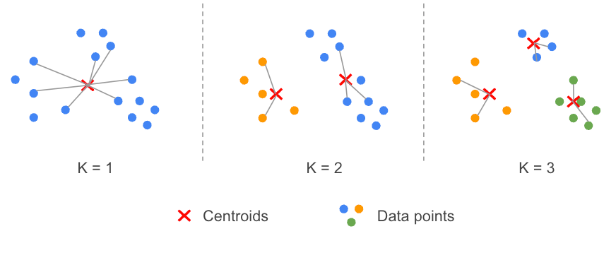
- STEP 1: Specify the number (K) of clusters to use.
- STEP 2: Randomly initialize (K) centroids.
- STEP 3: For each data point, calculate its distance with each centroid and assign the data point to the closest centroid.
- STEP 4: Compute the new centroid of each cluster (i.e. the mean of each variable).
- STEP 5: Execute STEP 3 again until the position of the centroids do not change (convergence).
The centroid of several continuous variables can be seen as the means of those variables, i.e. the data point that represents the centre of the cluster. It is important to keep in mind that convergence of centroids is not guaranteed and this should be considered when implementing such an algorithm.
When you discover the K-means algorithm for the first time, two questions may arise:
- How to choose the number of clusters (STEP 1)?
- Does the random initialization of centroids have an impact on the result (STEP 2)?
These two topics will be covered in the following sections.
K-means assumes that you know the number (K) of clusters you want to use to partition your dataset. The choice of K is therefore left to the person running the algorithm. Among the many techniques available, there are two main methods to help you choose the right value for K. Both are widely described on the web. To start, you might be interested by these two Medium articles:
- K-means Clustering: Algorithm, Applications, Evaluation Methods, and Drawbacks
- How to determine the optimal K for K-Means?
Again, I won’t focus too much on the formulas or code but rather on the explanations of the concepts.
The letter K in K-means represents the number of clusters that will be created by the algorithm. This number of clusters is defined by the analyst. K-means allocates data points to clusters by measuring distances between them and groups the closest together.
Principle of the Elbow method
This is an empirical method: the main idea is to run the K-means algorithm for a possible range of K values (e.g. from 1 to 10 clusters) and evaluate, for each scenario (K=1, K=2, …), the distance between the data points and their associated centroids (i.e. for each cluster).
For each run of the K-means algorithm, we actually compute the sum of the squared distance between each point and its closest centroid, this reminds us of the notion of variance. The sum of these quantities is called WCSS, Within-Cluster Sum of Square.
Intuitively, this quantity decreases when the number of clusters increases. Indeed, by increasing the number of centroids, we increase the chance of a data point to get closer to a centroid and therefore reduce its distance. The method aims to find the point (elbow) where adding more clusters does not bring value.
The challenge, as described in the many articles, is to determine when the number of K clusters is correct because we do not want to end up with too many clusters. Consequently, the best choice can be somewhat arbitrary.
Terminology sometimes used:
- Inertia: sum of squared distances of samples to their closest cluster centre (equivalent to WCSS).
- Distortion: average of the euclidean squared distance from the centroid of the respective clusters.
Silhouette analysis
The silhouette value is a measure of how similar an object is to its own cluster (cohesion) compared to other clusters (separation). -Wikipedia
The principle is as follows: if the number of clusters is correct, then the average distance between each data point within a cluster (often called “average intra-cluster distance”) should be smaller than the average distance with other data points from other clusters (“average inter-cluster distance”).
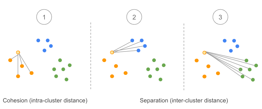
This method assumes that the data have been clustered. In other words, each data point is already assigned to a cluster. Let’s focus now on a given data point (in light orange on the image above) using an example of three clusters:
- We calculate the average distance of this point with all other data points in the same cluster. This is often noted as a(i).
- We calculate the average distance of the same point with all data points from other clusters. Let’s start with the blue cluster.
- We do the same calculation as step 2 but with the green cluster.
- We compare the results obtained in step 2 and step 3 and keep the minimum value because we do not really care which cluster is far away, but rather which one is near. To put it another way, we are interested in the neighbourhood of our considered data point. We denote this value b(i).
- Therefore, the silhouette value S for a given data point i is obtained by subtracting b(i) to a(i) and divide this quantity by the maximum value between a(i) and b(i). I tried to stay away from formulas, but sometimes it can be useful to see them:
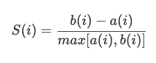
As a consequence, this value is always between -1 and 1.
b(i) and a(i) are always positive (average of distance), so if the average intra-cluster distance a(i) is greater than the average inter-cluster distance b(i) then S(i) will be negative. The data point under consideration is closer to another cluster. In this case , it appears misclassified.
If we extend this reasoning, when b(i) is very large compared to a(i), then S(i) will be close to 1: the data point is well classified.
When S(i) is about zero, the average intra-cluster distance is approximately equal to the average inter-cluster distance, the choice of assigning the data point to one cluster or another is not clear.
Selection of the best value for K
The average of the S(i) for all data points in a given cluster is called the average silhouette width of that cluster S(K). For each model (with 2, 3, 4, … K clusters) we can then calculate the average of S(K) — the cluster average silhouette width. This quantity is called the Average Silhouette Score. To select the best value of K, the score obtained must be as high as possible.
The two methods, Elbow and Silhouette, provide information from a different perspective. They are often used in combination to reinforce the choice of K. Another ally can sometimes support decision-making: the domain knowledge of the person performing the analysis!
While the decision to identify the right number of clusters is ultimately up to the analyst, different techniques exist to help the analyst to make informed decisions. The most popular are the Elbow method and the Silhouette analysis.
Initializing the centroids
The second facet of the algorithm that may concern you is the random choice of the initial centroids. Indeed, K-means is nondeterministic: the algorithm can produce different results depending on its initialization. Below are two different runs of the algorithm on the same dataset illustrating this:
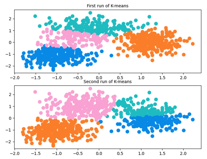
The purpose of this example is only to illustrate the fact that K-means can produce different results. Indeed, in this particular case, the number of clusters may not be appropriate. When K-means was run several times on this dataset but with only three clusters, the results were always consistent and identical. Moreover, as a best practice, it is recommended to run K-means several times to see the stability of the proposed clustering.
sklearn.cluster.KMeans allows you to select the way the first centroids are initialized. There are two options: random or K-means++. K-means++ is a technique of smart centroids initialization that speeds up the convergence of the algorithm. The main idea is to select initial centroids as far apart as possible.
The K-means algorithm can lead to different results, this is particularly true when the number of clusters is incorrect or when the pattern in the data is not clear.
Things to keep in mind
Importance of feature scaling
Feature scaling is essential for K-means to produce quality results. Because the algorithm relies on distance estimation, especially for the calculation of centroids, the different variables must be in the same range of magnitude.
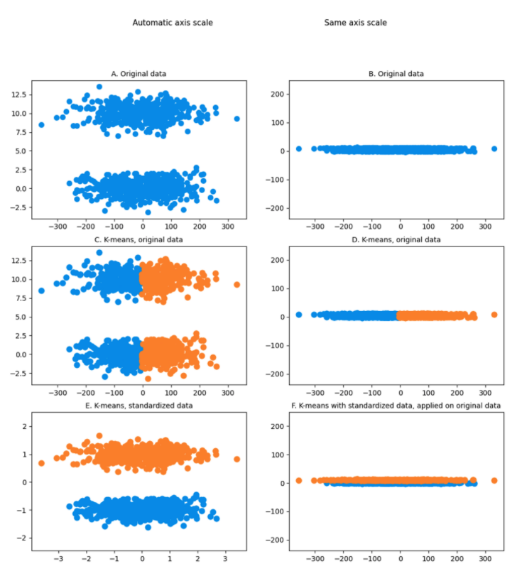
Below is an example of a dataset consisting of two obvious clusters (Chart A). It’s obvious because autoscaling lets you see it, but if this dataset is visualized on a graph with axes having the same scale (Chart B), this is no longer visible for either you or the algorithm.
It becomes even more interesting when you run K-means on this non-standardized dataset (Chart C and Chart D): two clusters are created containing half of each cloud of points. This is clearly the opposite of what you want to achieve!
Finally, when the dataset is standardized (Chart E and Chart F), the difference in scale appears and K-means is able to identify the true clusters.
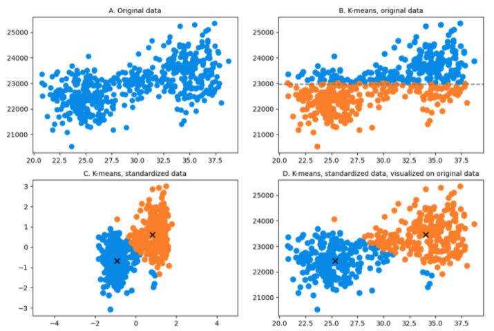
To be more concrete, suppose you want to perform a customer segmentation based on age and annual income. You have a dataset of 500 people between the ages of 20 and 40 shown in the figure below. Chart A represents this dataset (autoscaling) on which we can visually imagine two main clusters. Again, as explained above, they are visible because the two dimensions are not on the same scale otherwise, you would not be able to visualize it. When K-means is applied on the original data, the algorithm horizontally splits the data points in two groups. The reason for this is that when calculating distances, a 20-year change will compare the same as a change of $20 annual income. The euclidean distance used in K-means in STEP 3 of the algorithm between a possible data point A (23, 21000) and an hypothetic centroid K1 (25, 22500) will be:
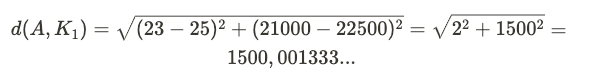
Thus, age does not weigh much in the calculation of the distance and, therefore, will not have a significant impact whether the person is 20 or 40. Consequently, K-means splits the clusters approximately following the mean of the annual income only, since that is the only dimension that really matters.
However, you want your algorithm to detect this age variation because it is an important factor in your study. Chart C and Chart D provide better clusters when the data is standardized before running K-means.
A final comment on this example is that you can see that some data points could be better categorized. This is due to the standardization effect but also because they may be outliers, which K-means is not good at dealing with.
Sensitivity to outliers
Since the algorithm minimizes distances between data points and centroids, outliers affect the position of the centroids and can shift cluster boundaries. However, dealing with outliers before running K-means can be challenging, especially on big datasets. Many attempts have been made to address the challenge of the outliers with K-means, but there does not seem to be a real consensus on an effective solution. Most of the time, using other algorithms K-medians, K-medoids or DBSCAN are preferred.
Categorical data
For the same reason as above, the fact that K-means minimizes the distance between data points and their nearest centroid, K-means is not relevant for categorical data. The distance between two categories, even though you encoded them as numbers, does not mean anything: there is no natural order between values. Other algorithms should be preferred.
Data pattern
The heart of the algorithm is based on the notion of centroid, so by design K-means always tries to find spherical clusters. The dataset containing a particular pattern might be difficult to capture for this algorithm. Algorithms such as DBSCAN are more suitable for detecting clusters of special data shapes. An illustration can be found here: DBSCAN clustering for data shapes k-means can’t handle well.
Since K-means is all about distance measurement, the algorithm is sensitive to outliers: they shift the centres of the clusters and thus the allocation of the data points.
Should managers be involved in technical considerations?
Recently, in a workshop organized by CERN IdeaSquare and Geneva Innovation Movement Association, we explored ways to reconcile the communication between high-level managers and technical experts while developing a product.
How can we optimize this collaboration to deliver faster and better solutions? While the event was fun (which can also be a parameter to consider), getting both parties around the same table to work on a common goal seemed to help a lot. In the specific case of data science, developing a data culture among the various stakeholders is certainly the way to go.
As mentioned earlier, I tried this with interesting feedback from a senior manager. Are you game? Why not spend 10 minutes in a meeting with high-level managers to demonstrate the selected model and how it behaves when playing with certain parameters? A script might be too crude, but with low-code/no-code software (such as Knime) it could trigger unexpected but interesting results.
Acknowledgements
- Sincere thanks to Sharon for her proofreading, suggestions and continuous support.
- Many thanks to Mathilde for her helpful comments and to Pauline for her artistic contribution!
A Deep Dive into K-means for the Less Technophile was originally published in Towards Data Science on Medium, where people are continuing the conversation by highlighting and responding to this story.
from Towards Data Science - Medium
https://towardsdatascience.com/a-deep-dive-into-k-means-for-the-less-technophile-eaea262bd51f?source=rss----7f60cf5620c9---4
via RiYo Analytics


ليست هناك تعليقات