https://ift.tt/JpjT1N5 Why do We use Cross-entropy in Deep Learning — Part 2 Explanation of one of the most widely used loss functions in ...
Why do We use Cross-entropy in Deep Learning — Part 2
Explanation of one of the most widely used loss functions in Artificial Neural Networks
Note. This is the continuation of the first part: Why do We use Cross-entropy in Deep Learning — Part 1
Entropy, Cross-entropy, Binary Cross-entropy, and Categorical Cross-entropy are crucial concepts in Deep Learning and one of the main loss functions used to build Neural Networks. All of them derive from the same concept: Entropy, which may be familiar to you from physics and chemistry. However, not many courses or articles explain the terms in-depth, since it requires some time and mathematics to do it correctly.
In the first post, I presented three different but related conceptions of entropy and where its formula derives from. However, there is still one key concept to address, since Deep Learning does not use Entropy but a close relative of it called Cross-entropy. What this term means, how to interpret it and on which Deep Learning problems it is applied is the focus of this post.

Cross-Entropy
Recalling the first post (link), the entropy formula can be interpreted as the optimal average length of an encoded message.

Note1. Recall from the previous post that the base of the logarithm isn’t really important, since changing a logarithm base is equivalent to multiplying by a constant. This only applies to optimization and comparative methods, where constants are ignored.
Alternative to entropy, Cross-entropy is defined as the entropy of a random variable X, encoded using a probability distribution P(x), but using a different probability distribution Q(x) to compute the average.
In other words, what would be the optimal average message length of a random variable X distributed as Q(x) but using the encoding system of the distribution P(x)?

Note2. Another common notation to define Cross-entropy is H(Q,P). However, I consider using sub-indices instead in order to keep the notation consistent with the Entropy formula.
To clear things up, let’s use an example. I am going to take the same example as in the first post, but remember that it works the same with any discrete random variable.
In the example, we were studying the optimal average length of encoding our laboratory experiments which could result in 6 different outcomes (microstates): Microstate 1 (M1), M2, …, M6.
Let’s suppose now that we have some parameters K that we can modify in our experiment so that when we use different combinations of K we obtain different probability distributions for the results (the microstates)
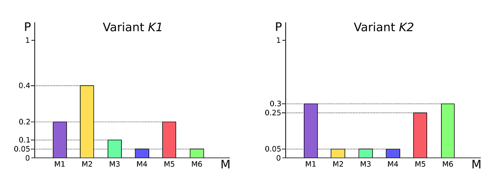
As we have seen, entropy is a function of a probability distribution, i.e. the entropy of a distribution P(x) and Q(x) does not have to be the same. The reason is that to calculate entropy we have set the respective probabilities of each result as the cost value (see section Entropy Formula of the first part for a detailed explanation) In other words, the encoding for P(x) isn’t necessarily the same as the encoding of Q(x). Although X is the same random variable for both cases, what changes is its distribution.
Now the following dilemma emerges: If we could only use one encoding system to send the results of experiment variants K1 and K2, which encoding would be more optimal, and therefore should we use? Encoding K1 or K2?
The solution to this problem goes through computing the Entropy and Cross-entropy for each variant K1 and K2 (with respect to the other) and averaging the results to obtain the global average length using encoding systems K1 and K2.
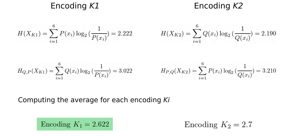
As calculated, the optimal coding system for sending messages of the K1 and K2 variants is the one from K1, which produces the shortest length (2.622).
One might think that the difference between the two encodings isn’t so significant, as the results have to be rounded up when working with bits. However, when the sequences of words included in the message are sufficiently high, this difference is palpable.
Suppose your message it’s a tweet with 280 bits maximum. With encoding K1 you will be able to send 280/2.622 ~ 106 words on average, whereas using encoding K2 enables you to communicate 103 words (Who hasn’t ever suffered from not being able to write 3 more words in a tweet?) And the gap continues to grow as you increase the number of words per message.
Note3. Furthermore, there is a concept called fractional bits, which is a method of maximizing the optimal length of words when communicating more than one word whose optimal length is decimal.
An important observation is that Cross-entropy isn’t symmetric, so that

Cross-entropy in Deep Learning
We have already seen an example of how we can apply Cross-entropy to a problem, but since Deep Learning is not very interested in (just) encoding messages, why, when, and how did this function come into the scene?
The answer, of course, lies in its application, so let’s introduce the problem Cross-entropy solves in Deep Learning.
Deep Learning for classification tasks
Imagine you want to classify electrocardiogram signals (ECM) into a set of different patterns that represent cardiovascular diseases. Actually, this is a very difficult task even for the most experimented cardiologists since patterns of cardiac abnormalities can be very subtle and the difference between a healthy person and a person with cardiac disease is minimal.
Note4. If you are interested in how the classification of ECM is tackled nowadays using Deep Learning refer to this article.
Forcing the model to just predict an integer from 1 to K, where K is the number of classes (ECM patterns), isn’t a good tactic. Using this system, the error of our model would be “absolute”, in the sense that we would be able to tell if the model has performed well or badly, but not how bad or how good it has been in its prediction.
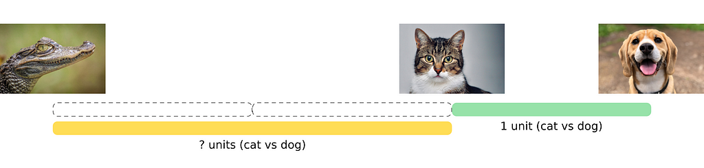
Suppose the model has predicted class 2 but the correct result is class 4, then how can we compute the error? Calculating the distance (or the MSE) between correct and predicted class (|4–2| = 2) can’t be used as an error measurement, because then we are stating that predicting class 2 is better than predicting class 9 (|4–2| < |4–9|), that is, we are assuming that class 2 is closer to class 4 than is class 9 based on our human criteria. Moreover, this method also assumes that class 3 is as close to class 4 as it is to class 2, which in practice is not possible to evaluate: How similar are a crocodile, a cat, and a dog? Perhaps a cat is 1 unit similar to a dog, but then how many units cat vs dog are the crocodile similar to the cat? We can’t simply do it because we cannot compare a crocodile vs a cat using a cat vs dog measurement unit!
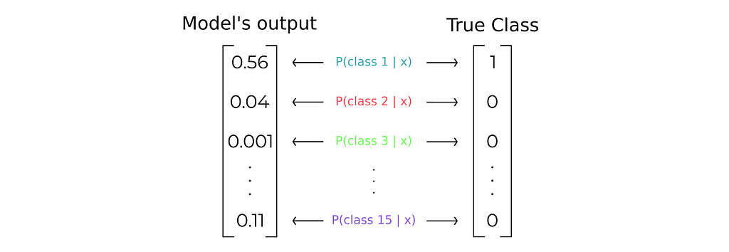
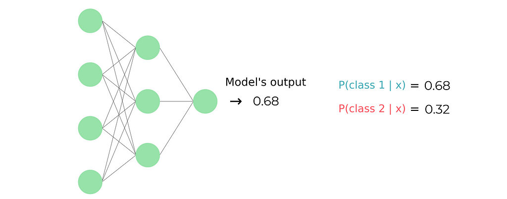
Another way of thinking of the problem is probabilistic, where instead of outputting 1,2 or K, the model will estimate the probability of the ECM presenting each pattern.
The output of our network will be then a probability distribution over all the K classes
Thus, the ECM pattern with a probability greater than >0.5 will be the pattern that the network has classified in the input ECM signal.
Note5. This simple and intuitive assumption of assigning a data sample to its most likely class where P(class k | x) is the greater (reads probability of belonging to class k given the data sample x) comes from the notion of Naive Bayes Classifier which in an ideal world where we know the true underlying conditioned probabilities is the best possible classifier.
To compute now the error we must also define a probability distribution for the expected output (i.e. the true class) Since we want to define probability 1 to the correct class and probability 0 to the rest, it is as simple as using one-hot encoding. Therefore, class 1 will be [1 0 0 … 0], class 2 [0 1 0 … 0], and so on.
Categorical Cross-Entropy
At this point, We have defined the problem approach and the form of the model’s output, but we haven’t established any loss function yet.
We need to find a way of measuring the difference between the model’s output and the true class vector i.e. we need to define a measure of the distance between two probability distributions.
Not surprisingly mathematicians had already thought about a tool capable of solving this need. The solution lies in the field of Information Geometry under the concept of Divergence
`In information geometry, a divergence is a kind of statistical distance: a binary function which establishes the separation from one probability distribution to another on a statistical manifold (a space where each point represents a probability distribution) (Wikipedia)
There are currently different divergence measurements (see), however, one of them is very special because it significantly simplifies the calculations for us: The Kullback–Leibler divergence.

It is important to note that the Kullback-Leibler divergence isn’t symmetric:

Since we are using the the Kullback-Leibler divergence as an error measurement (the more the distance between the probab. distributions the worse the model’s prediction), we want to minimize it.
Note6. The following derivation is taken from this video.
Defining :
P* → The True Class distribution
P → The predicted Model distribution
θ → The Model parameters
P*(y|x) → The true probability of belonging to y class given the input data x
P(y|x;θ) → The predicted probability by the model of belonging to y class given the input data x and the parameters θ

And operating the terms:
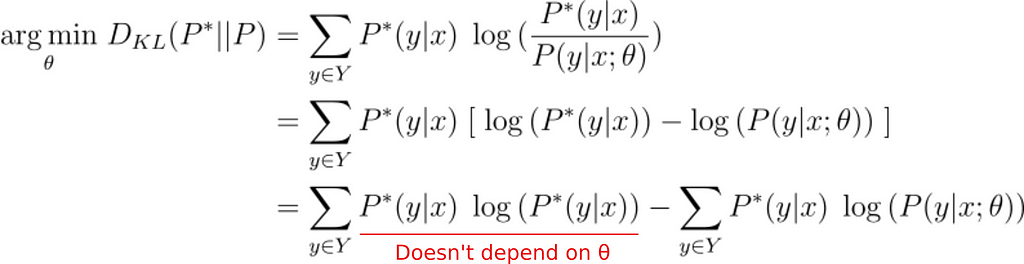
Finally, we can show that:
Minimizing the Kullback-Leibler divergence is equivalent to minimizing the Cross-entropy between the True class probability distribution (P*) and the predicted (P)

That is, in optimization problems Cross-entropy can be seen as a measure of the distance between two probability distributions.
Note7. We can also think about computing the KL Divergence D_{KL}(P||P^*) since as we know KL is not symmetric. However, doing that leads to a mathematical indeterminacy. After operating the terms and removing the ones not dependent on θ, we get the formula described below. The indeterminacy occurs when P*(y|x) = 0 (remember P*(y|x) is a one-hot encoding vector) and log(0) is not defined.

Computing Cross-entropy alongside multiple classes receives the name of Categorical Cross-entropy to differentiate from Binary Cross-entropy. In Deep Learning libraries like Tensorflow there already exists a pre-built function to compute the Categorical Cross-entropy:
tf.keras.losses.CategoricalCrossentropy()
Binary Cross-Entropy
In the previous problem we had to classify a data point x into multiple classes, but what about binary classification problems where we just have 2 classes?
Again we can think of the problem using probabilities. The only difference is that now the output of our model isn’t a probability vector rather than a single value representing the probability of the input data point x of belonging to the first class, since we can compute the probability of belonging to the second class by applying P(class 2) = 1-P(class 1)
Once again we can apply the Cross-entropy formula. Using now the fact that we have just two classes we can expand the summation:

Nevertheless, a fact that I haven’t mentioned before is that usually loss functions are computed on a batch of data points, so the average loss is taken over those points. Then, you will probably see Binary Cross-entropy (BCE) as:

Likewise Categorical Cross-entropy, most Deep Learning libraries have a pre-built function for Binary Cross-entropy. In the case of Tensorflow:
tf.keras.losses.BinaryCrossentropy()
Conclusions
So far during this series of two posts I’ve presented the intuition and formal derivation of Entropy, Cross-entropy, Categorical Cross-entropy and Binary Cross-entropy, as well as their application in classification problems. Summarizing all the content seen in a few lines:
- (Shannon) Entropy = Optimal average length of an encoded message, where the base of logarithm in the formula defines the possible characters for encoding (2 for binary code)
- Cross-entropy = The optimal average message length of a random variable X distributed as Q(x) but using the encoding system of the distribution P(x) → In optimization problems can be seen as a measure of the distance between two probability distributions
- Categorical Cross-entropy = Cross-entropy applied as a loss function in multiclassification problems (when there are more than 2 classes)
- Binary Cross-entropy = Cross-entropy applied as a loss function in binary classification problems (when there are just 2 classes)
Finally, if you want to read more on how classification is performed using Neural Network models, I recommend reading my post Sigmoid and SoftMax Functions in 5 minutes, in which I explain the two activation functions used for outputting the probability distributions in both multiclass and binary problems.
Sigmoid and SoftMax Functions in 5 minutes
Why do We use Cross-entropy in Deep Learning — Part 2 was originally published in Towards Data Science on Medium, where people are continuing the conversation by highlighting and responding to this story.
from Towards Data Science - Medium
https://towardsdatascience.com/why-do-we-use-cross-entropy-in-deep-learning-part-2-943c915db115?source=rss----7f60cf5620c9---4
via RiYo Analytics


ليست هناك تعليقات