https://ift.tt/I8W2PNx Using SHAP with Cross-Validation in Python Making AI not only explainable but also robust Photo from Michael Dzie...
Using SHAP with Cross-Validation in Python
Making AI not only explainable but also robust

Introduction
In many situations, machine learning models are preferred over traditional linear models because of their superior predictive performance and their ability to handle complex nonlinear data. However, a common criticism of machine learning models is their lack of interpretability. For example, ensemble methods such as XGBoost and Random Forest, combine the results of many individual learners to generate their results. Although this often leads to superior performance, it makes it hard to know the contribution of each feature in the dataset to the output.
To get around this, explainable AI (xAI) has been conceived and is growing in popularity. The xAI field aims to explain how such unexplainable models (so-called black-box models) made their prediction, allowing the best of both world: prediction accuracy and explainability. The motivation for this is that many real-world applications of machine learning require not just good predictive performance but also an explanation of how the results were generated. For example, in the medical field where lives may be lost or saved based on decisions made by a model, it is important to know what the drivers of the decision were. Additionally, being able to identify important variables can be informative for identifying mechanisms or treatment avenues.
One of the most popular and effective xAI techniques is SHAP. The SHAP concept was introduced in 2017 by Lundberg & Lee but actually builds on Shapley values from game theory, which existed long before. Briefly, SHAP values work by calculating the marginal contribution of each feature by looking at the prediction (per observation) in many models with and without the feature, weighting this contribution in each of these reduced feature set models, and then summing the weighted contribution of all of these instances. Those who would appreciate a more thorough description can see the links above, but for our purposes here it suffices to say: the larger the absolute SHAP value for an observation, the larger the effect on the prediction. It thus follows that the larger the average of the absolute SHAP values for all observations for a given feature, the more important the feature is.
Implementing SHAP values in Python is easy with the SHAP library, and many walkthroughs already exist online explaining how this can be done. However, I found two major shortcomings in all of the guides that I came across for incorporating SHAP values into Python code.
The first is that most of the guides use SHAP values on basic train/test splits but not on cross-validation (see Figure 1). Using cross-validation gives a much better idea about the generalizability of your results, whereas the results from a simple train/test split are liable to drastic changes based on how the data is partitioned. As I explain in my recent article on “Machine learning in Nutrition Research”, cross-validation should almost always be preferred over train/test split, unless the dataset you are dealing with is huge.
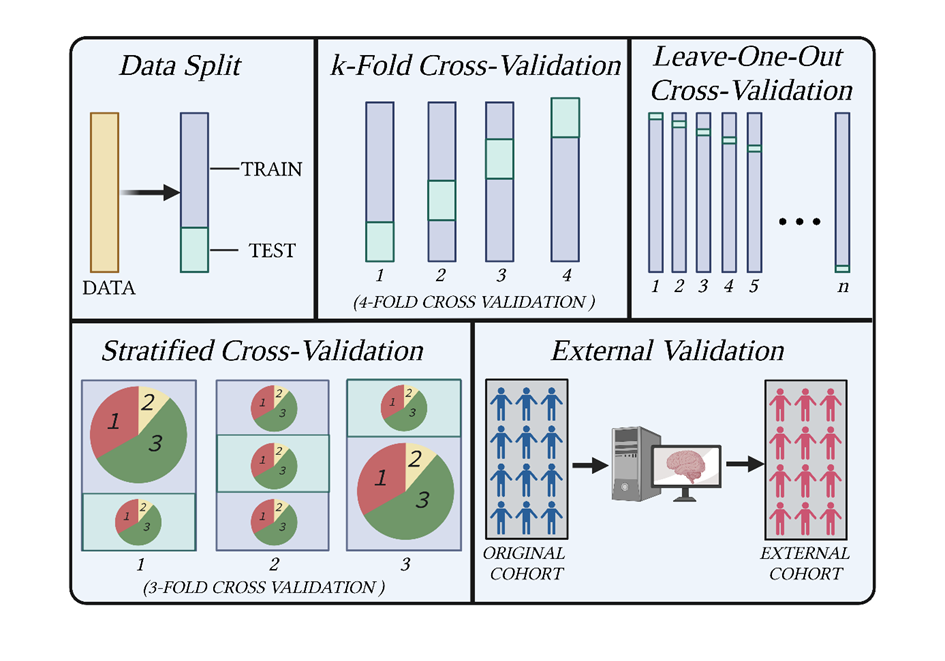
The other shortcoming is that none of the guides I came across used multiple repeats of cross-validation to derive their SHAP values. Whilst cross-validation is a big improvement on a simple train/test split, it should ideally be repeated multiple times using different splits of the data each time. This is especially important with smaller datasets where the results can change greatly depending on how the data is split. This is why it is often advocated to repeat cross-validation 100x in order to have confidence in your results.
To deal with these shortcomings, I decided to write some code to implement this myself. This walk-through will show you how to get SHAP values for multiple repeats of cross-validation and in corporate a nested cross-validation scheme. For our model dataset, we will use the Boston Housing dataset, and our algorithm of choice will be the powerful but uninterpretable Random Forest.
Implementation of SHAP Values
Whenever you’re building code with various loops as we will be, it usually makes sense to start with the innermost loop and work outwards. By trying to start from the outside and build the code in the order it will also run, it’s easier to get confused and also harder to troubleshoot when things go wrong.
Thus, we start with the basic implementation of SHAP values. I will presume you’re familiar with the general use of SHAP and what the code for its implementation looks like, so I won’t spend too long on an explanation. I leave comments throughout (as is always good to do) so you can check those, and if you’re still unsure then check out the links in the introduction or the docs of the library. I also import libraries as they’re used rather than all at once at the start, just to help with intuition.
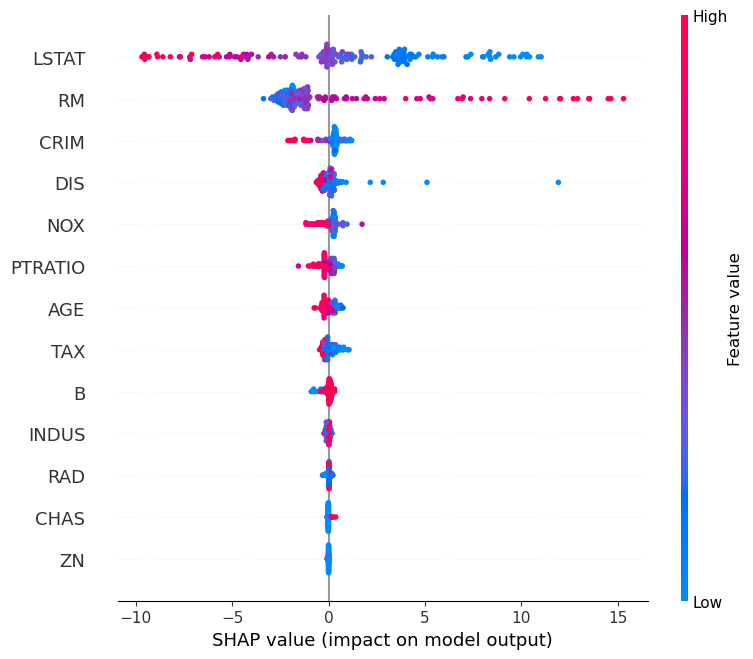
Incorporating Cross-Validation with SHAP Values
We are most often used to seeing cross-validation implemented in an automated fashion by using sklearn’s cross_val_score or similar. The problem with this is everything happens behind the scenes, and we don’t have access to the data from each fold. Of course, if we want to get SHAP values for all our data points, we need to access each data point (recall that every data point is used exactly one time in the test set and k-1 times in training). To get around this, we can use KFold in combination with .split.
By looping through our KFold object with .split, we can get the training and test indices of each fold. Here, fold is a tuple, where fold[0] is the training indices and fold[1] is the test indices of each fold.
Now, we can use this to select the training and test data from our original data frame ourselves, and thus also extract the information we want. We do this by making a new for loop and to get the training and test indices of each fold, and then simply performing our regression and SHAP procedure as normal. We then only need to add an empty list outside of the loops to keep track of the SHAP values per sample and then append these at the end of the loop. I use #-#-# to denote these new additions:
Now, we have SHAP values for every sample, instead of just samples in one test split of the data, and we can plot these easily using the SHAP library. We first just have to update the index of X to match the order in which they appear in each test set of each fold, otherwise, the color-coded feature values will be all wrong. Notice that we re-order X within the summary_plot function so that we don’t save our changes to the original X data frame.
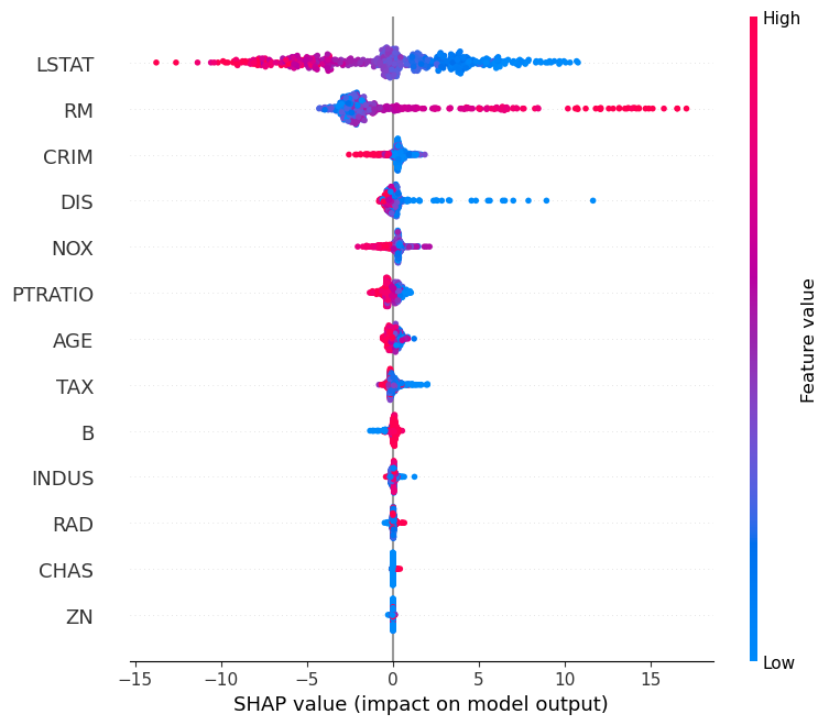
We can see from the plot that there are now many more data points (all of them, in fact) compared to when we just use a train/test split. Already, this improves our procedure since we get to make use of the entire dataset instead of just a portion.
But we still have no idea about stability — i.e., how the results would change had the data been split differently. Fortunately, code our way out of this problem below.
Repeating Cross-Validation
Using cross-validation greatly increases the robustness of your work, especially with smaller datasets. If we really want to do good data science, however, cross-validation should be repeated over many different splits of the data.
First of all, we need now need to consider not just the SHAP values of each fold, but also the SHAP values of each fold for each repeat and then combine them to plot on one graph. Dictionaries are powerful tools in Python, and this is what we will be using to track the SHAP values of each sample in each fold.
First, we decide how many cross-validation repeats we want to perform and then establish a dictionary that will store the SHAP values of each sample for each repeat. This is achieved by looping through all of the samples in our dataset and creating a key for them in our empty dictionary, and then within each sample creating another key to represent the cross-validation repeat.
Then, we add some new lines to our existing code that allow us to repeat the cross-validation procedure CV_repeats number of times and add the SHAP values of each repeat to our dictionary. This is achieved easily by updating some lines at end of the code so that instead of appending a list of the SHAP values per sample to a list, we now update the dictionary. (Note: collecting test scores per fold is probably also relevant, and although we don’t do that here because the focus is on using SHAP values, this can be easily updated by adding another dictionary, with CV repeats as the keys and test scores as the values).
The code looks like this, with #-#-# denoting upates to the existing code:
To visualize this, let’s say we want to check the fifth cross-validation repeat of the sample with index number 10, we just write:
where the first square bracket denotes the sample number and the second denotes the repeat number. The output is the SHAP values for each of the columns in X for sample number 10 after the fifth cross-validation repeat.
To see the SHAP values of all the cross-validation repeats of one individual, we would just type the number in the first square bracket:
However, this is not really much use to us (other than for troubleshooting purposes). What we really need is a plot to visualize this.
We first need to average the SHAP values per sample per cross-validation repeat into one value for plotting (you could also use the median or other statistics if you preferred). Taking the average is convenient but can hide variability within the data that might also be relevant to know. Thus, while we’re taking the average we will also get other statistics, such as the minimum, the maximum, and the standard deviation:
The above code says: for each sample index in our original data frame, make a data frame from each list of SHAP values (i.e., each cross-validation repeat). This data frame contains each cross-validation repeat as a row and each X variable as a column. We now take the average, standard deviation, min, and max of each column by using the appropriate functions and using axis = 1 to perform the calculations column-wise. We then convert each of these to data frames
Now, we simply plot the average values as we would plot the usual values. We also don’t need to re-order the index here because we take the SHAP values from our dictionary, which is in the same order as X.
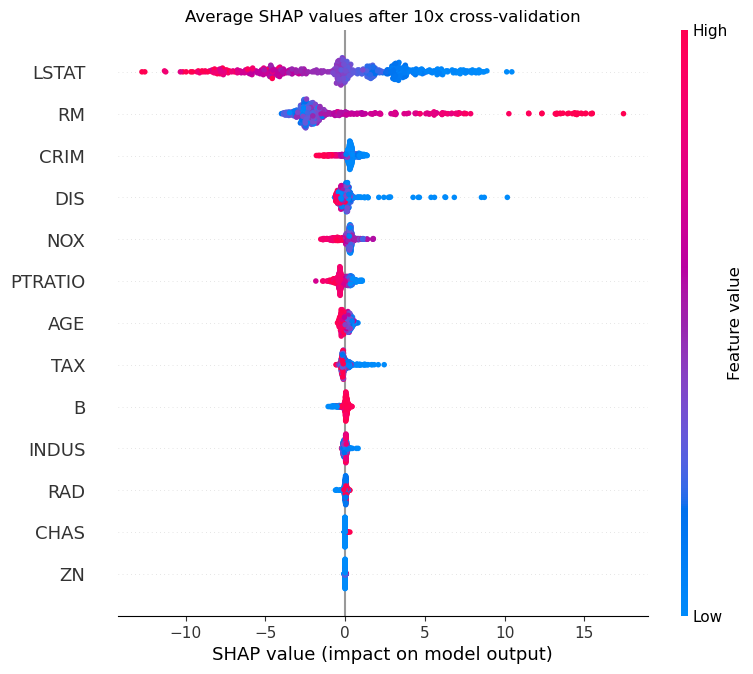
Since our results have been averaged over many repeats of cross-validation, they are more robust and trustworthy than a simple train/test split performed only once. However, you may be disappointed if you compare the plots before and after and see that, other than the extra data points, not much changes. But don’t forget, we’re using a model data set which is nice and tidy with well-behaved features that have strong relationships with the outcome. In less utopic circumstances, techniques like repeated cross-validation will expose the instability of real-world data in terms of results and feature importance.
If we wanted to beef up our results even more (which of course we do) we could add some plots to get an idea about the variability of our proposed feature importances. This is relevant because taking the average SHAP value per sample might mask how much they change with different splits of the data.
To do this, we have to convert our data frame to long form, after which we can make a catplot using the seaborn library
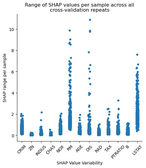
In the catplot above, we see the range (maximum value — minimum value) across each repeat of CV repeats for each sample. Ideally, we would want the values on the Y-axis to be as small as possible, since this which imply more consistent feature importances.
We should keep in mind though that this variability is also sensitive to the absolute feature importance, i.e., features deemed more important will naturally have data points with larger ranges. We can partially account for this by scaling the data.
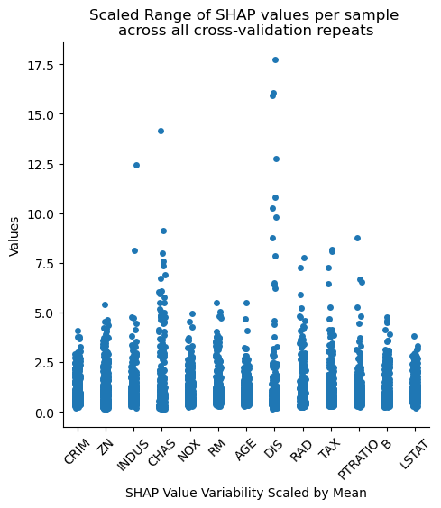
Notice how different things look for LSTAT and RM, two of our most important features. Now we get a better reflection of variability scaled by the overall importance of the feature, which may or may not be more relevant depending on our research question.
We could conjure up similar plots based on the other statistics that we collected, such as standard deviation, for example.
Nested Cross-Validation
All this is great, but one thing is missing: our random forest is in its default mode. Although it performs pretty well on this data set with the default parameters, this might not be the case in other situations. And besides, why should we not try to maximize our results?
We should be careful not to fall into a trap that seems to be all too common in machine learning examples these days which is to optimize the model hyperparameters on data that is also present in the test set. With a simple train/test split, this is easy to avoid — you simply optimize the hyperparameters on the training data.
But as soon as cross-validation enters the equation, this concept seems to be forgotten. Indeed, all too often people use cross-validation to optimize hyperparameters, and then use cross-validation to score the model. In this case, data leakage has occurred, and our results will be (even if only slightly) over-optimistic.
Nested cross-validation is our solution to this. It involves taking each of the training folds from our normal cross-validation scheme (called here the “outer loop”) and optimizing hyperparameters by using another cross-validation on the training data of each fold (called the “inner loop”). This means that we optimize the hyperparameters on training data and then can still get a less biased idea about how well the optimized models perform on unseen data.
The concept can be a bit tricky to understand, but for those wishing for a little more detail, I explain it my article linked above. In any case, the code is not so difficult, and reading through it will probably help with comprehension. And in fact, we already have much of the code prepared during our process above, and only small tweaks are required. Let’s see it in action.
The main consideration with nested cross-validation — especially with many repeats as we use — is it takes a lot of time to run. For that reason, we will keep our parameter space small and use a randomized search rather than grid search (though random search often performs adequately in most situations anyway). If you did want to be more thorough, you might need to reserve some time on a HPC. Anyway, outside of our initial for loop we will establish the parameter space:
We then make the following changes to the original code:
- CV will now become cv_outer because, since we now have two cross-validations, we need refer to each appropriately
- Inside our for loop in which we loop through the training and test IDs, we add our inner cross-validation scheme, cv_inner
- Then, we use RandomizedSearchCV to optimize our model on inner_cv, select our best model, and then use the best model to derive SHAP values from the test data (the test data here being the outer fold test).
And that’s it. For demonstration purposes, we reduce CV_repeats to 2 since otherwise, we could be here a while. Under real circumstances, you’d want to keep this high enough to maintain robust results with also optimal parameters, for which you might not a HPC (or a lot of patience).
See the code below for these changes, again with #-#-# denoting new additions.
Conclusion
The ability to explain complex AI models is becoming increasingly important. SHAP values are a great way to do this, however, the results of single training/test splits cannot always be trusted, especially in smaller datasets. By repeating procedures such as (nested) cross-validation multiple times, you increase the robustness of your results and can better gauge how your results might change if the underlying data also changed.
Note: All uncredited images are my own.
Using SHAP with Cross-Validation was originally published in Towards Data Science on Medium, where people are continuing the conversation by highlighting and responding to this story.
from Towards Data Science - Medium
https://towardsdatascience.com/using-shap-with-cross-validation-d24af548fadc?source=rss----7f60cf5620c9---4
via RiYo Analytics

No comments