https://ift.tt/IA5tZig A use case of indoor temperature modelization to choose the optimal heating power Physics-guided machine learning ...
A use case of indoor temperature modelization to choose the optimal heating power
Physics-guided machine learning
While machine learning has shown tremendous success in many scientific domains, it remains a grand challenge to follow basic physics laws. Multiple examples have shown that merely data-driven solutions fail to follow the physics laws. At the same time, some developed even mature theories in science would help guide AI to converge to a better solution that makes sense physically.
At the same time, the majority of physical models do not provide any framework of uncertainty while uncertainty quantification methods in machine learning help to introduce uncertainty to the existing physics laws that might help us to understand correlations or even casual relations hidden in the data and complex dynamics not fully captured by simplified physical/mathematical models.
This post aims to demonstrate that incorporating the physics constraints in the a data-driven estimation model for prediction and uncertainty quantification is a promising approach to improve model performance.
The example in the coming article focuses on an uncertainty prediction of indoor temperature modelized by a physics-guided machine learning model.
Physical model of indoor temperature
I need to buy a new heater for my house after the old one was broken. What is the power that I need? Too big, a waste of power; too small, cannot heat enough .This question is worth asking in the context of the ongoing global energy crisis and climate change no matter from the purpose of protecting the environment or saving money.
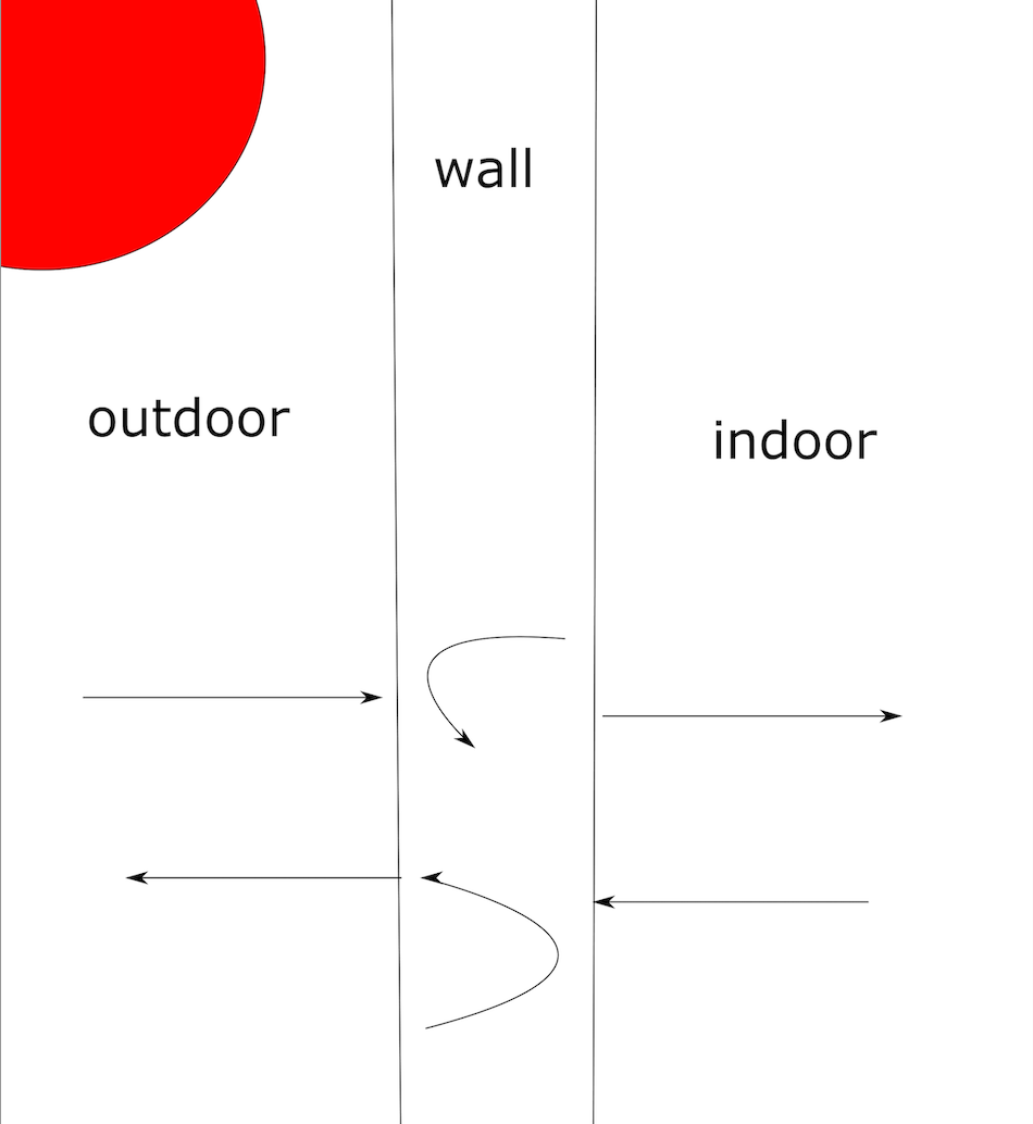
Before answering the question, we need to understand the dynamics of the temperatures. Let us suppose that heat is transferred between the indoor air and the wall which can store an important quantity of energy. In the mean time, the heat is also being transferred between the wall and the outdoor air. See the plot below for an illustration.

The indoor temperature, together with the wall temperature and the outdoor temperature, can be described by the following ordinary differential equation (ODE) given by the Newton’s cooling law:

where T_{in}, T_{wall}, T_{out} are the indoor, wall, outdoor temperature, C_{in}, C_{wall} the heat capacity (KJ/K) of the indoor air and the wall and U_{wall}, U_{out} the heat transfer coefficients (KW/K) of the wall and the outdoor air. Here, P is the power of the heating system. Of course, when the heating is off in the house, the equation turns to:

The equation above is easy to understand: the rate of temperature change is proportional to the temperature difference and is determined by both heat transfer and the heat capacity of different bodies in the system.
If we want to evaluate the minimal value of P, that is, the heating power the house should have, we have to know the values of the heat capacity and the heat transfer coefficient.
Bayesian modelization of indoor temperature
Note that uncertainty is inevitable when we measure different bodies’ temperatures, we would build a network of the indoor temperature dynamics along with Bayesian inference to learn the posterior of the concerning parameters. We would like to build a model as followings:
- Discritizied the ODE with a classic Runge-Kutta integration, a numerical method involving successive approximations for the resolution of ODEs with the form of dy/dx=f(x,y).
- With the given prior of parameters, use Markov chain Monte Carlo (MCMC) to learn the posteriors. This step can be realized by the package pymc.
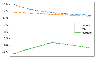
The model would be trained on a dataset of temperatures measured every 5 minutes during 24 hours in my room where I was trembling all day because the heating was off :( Both indoor and outdoor temperatures were measured every five minutes. The hourly outdoor temperature was obtained from MeteoFrance and was interpolated to have the time granularity every 5 minutes.

Python implementation
The implementation of this post can be found in the notebook. Let us take a quick look of the key part of the implementation:
The code contains three parts:
- Line 6-12 defines the prior of the parameters: the heat capacity, the heat transfer coefficients and the noise of temperatures. Remark that I rescale the values for the corret order of magnitude.
- Line 14- 35 uses the Runge-kutta method to update the values of the vector y_mean which would be used later.
- Line 37 defines a normal distribution whose mean is the y_mean. This normal distribution will be used in the sampling to learn all the parameters.
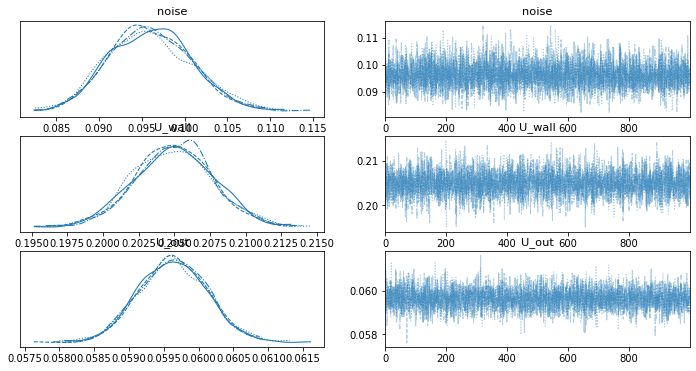
Now let pymc do its job by drawing samples from the posterior. Here is the traceplot of U_{wall}, U_{out} and the noise that we wanted to learn.

The question that what heating power I need is now evident to answer: imagine that in the worse case, my house has 10-celsius degrees less than that of the wall, and I would need a minimal heating power of about 2.1KW with 95% confidence.
Conclusion
In this post, we used a simple indoor temperature to demonstrate how physics laws can guide a data-driven machine learning model to get a good performance in uncertainty prediction. The author would like to argue that this method gives a promising approach to incorporating existing developed theories into artificial intelligence and would introduce cross-domain collaborations to improve the performance of many estimation models.
I am looking forward to your feedback and deeper discussions.
Physics-guided machine learning model for uncertainty prediction was originally published in Towards Data Science on Medium, where people are continuing the conversation by highlighting and responding to this story.
from Towards Data Science - Medium
https://towardsdatascience.com/physics-guided-machine-learning-model-for-uncertainty-prediction-1e3b733fd798?source=rss----7f60cf5620c9---4
via RiYo Analytics

No comments