https://ift.tt/QxVXvrl Unraveling microstructural features by FFT Photo by Matthew Henry on Unsplash Background All energies in this...
Unraveling microstructural features by FFT

Background
All energies in this universe have particle-wave dual characteristics. Fourier series and Fourier transform are widely used mathematical operations that decompose wave signals from different energies to extract valuable data. While solving a problem on heat conduction, French mathematician Joseph Fourier analyzed the sinusoidal components of heat waves, which led to the development of the Fourier series and Fourier analysis.
Although these mathematical operations mostly find usage in processing electromagnetic radiations such as radio, audio and electrical signals, they are also extensively applied in image processing to gather information. Signals generated from electromagnetic radiations are time-dependent, while that from images are space-dependent.
Here I will discuss why and how the Fourier transform is instrumental in interpreting images. And being a materials scientist, I will specifically highlight this tool’s strength in materials characterization.
I will begin with a brief overview of the Fourier series and the Fourier transform for ease of understanding this post.
A short introduction to the Fourier series, Fourier transform and Fast Fourier transform (FFT)
A Fourier series is a sum that represents a periodic function as a sum of sine and cosine waves. Here is the equation describing the series.
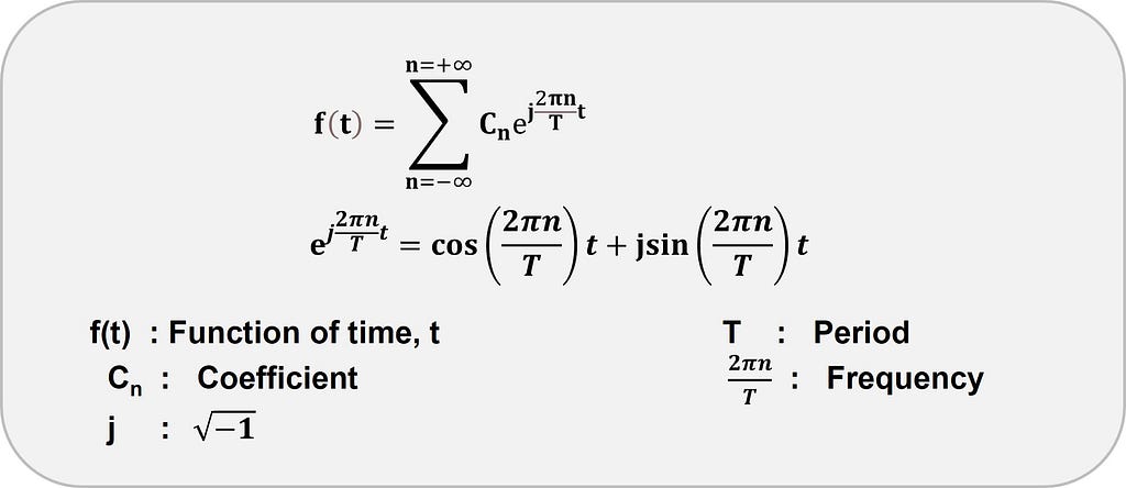
A periodic function repeats at regular intervals called time periods. For instance, the below function f(x) repeats itself at a regular interval of 2π:
f(x) = sin(x)
Frequency is the inverse of a period.
The Fourier transform operation transforms a signal in the time domain into the frequency domain or spatial domain into the spatial frequency domain (also known as reciprocal space) and is represented by the below equations.
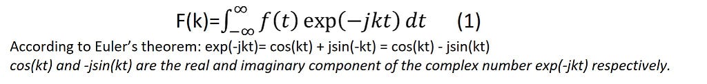

F(k ) is a function of frequency k; j is the imaginary number √-1. The above equations represent continuous Fourier transforms since the frequency and time (or spatial coordinates) variables are continuous-valued, varying from -∞ to +∞. In addition, we can also apply the transform operator over discrete points/samples, and the operation is called Discrete Fourier Transform (DFT). DFT transforms the continuous integral (Eq. 2) into a discrete sum:

Evaluation of the sum over N points or samples involves computational complexity proportional to O(N²) where O represents the order of complexity. Cooley and Tukey in 1965 implemented the divide-and-conquer algorithm (O(NlogN)) to accelerate the evaluation of the sum (Eq. 3). Cooley-Tukey algorithm is the first implementation of FFT. Frigo and Johnson at MIT further developed the FFT algorithm and created FFTW (Fastest Fourier Transform in the West) which is widely used worldwide. (Note: pyFFTW is the pythonic wrapper around FFTW).
Let us now understand how we can use FFT to analyze digital images.
Relevance of FFT in Digital Images
A digital image is composed of basic units called pixels, and each pixel is assigned a particular value of intensity varying between 0 and 255. The spatial domain of an image contains information on pixel intensity and pixel coordinates in real space.
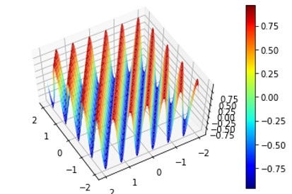
Now let’s generate an image, as shown below, from a 2D periodic function f(x,y) = sin(2πx +3πy) using NumPy.
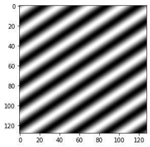
The corresponding 3D representation of the image beautifully captures the wave characteristics, thereby justifying the Fourier transform operations on images. Thus, processing the image signals by Fourier transform can unearth hidden but essential data for scientists and engineers.
Click here to learn about generating images from functions in Python.
FFT for Microstructure processing
In materials science, micrographs are the images of interest to explore and excavate data that will eventually impact a material’s performance.
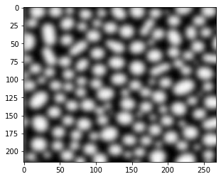
Let me now demonstrate an image (micrograph) processing to retrieve precise edges of microstructural features using a Fourier filter. I have considered a defocussed image (shown below) displaying roundish particles whose edges cannot be identified accurately.
I have used the FFT library of NumPy to write codes for image processing. (You can use pyFFTW and compare the relative execution times. When does pyFFTW beat numpy.fft?)
Here, I am writing the major steps involved when you apply FFT to the image above:
‣ I used imread to convert the jpg file of the image to a matrix (A ) whose elements store the information about each pixel (its coordinates and intensity).
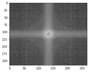
‣ Transformation from real space to Fourier space: I apply np.fft.fft2 function to the image matrix A to transform it from real (spatial) to frequency domain followed by shifting back the off-centered zero frequency components to the center. The code output looks like this 👇:
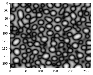
‣ Masked image: Since the edges of particles correspond to high frequency, a mask, allowing only such frequencies to pass through, is applied to the transformed image obtained from the previous step. This helps in highlighting the edges.
‣ Final Filtered image: Finally, we need to get back to the real space from spatial frequency space by deploying np.fft.ifft2 function to the masked image. I have shared below the processed image with distinct edges of the particles. One can easily measure the size of particles with defined boundaries.
A comparison with other image processing filters
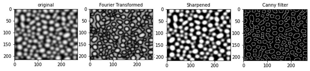
For a comparative study, I have applied two other image filters — Canny and unsharp masking filters on the above micrograph.
As seen clearly (displayed below), the Fourier filter outperforms the Canny and unsharp masking filters to identify the edges of the particles for precise measurement. The Fourier filter gets an advantage due to its ability to deconvolute a signal accurately in terms of its amplitude, frequency, orientation and phase.
Click here to view the entire code.
Key takeaways
✓ The Fourier series can be applied only to periodic functions, while the Fourier transform tool operates on non-periodic functions too.
✓ Images are mostly non-periodic. However, Fourier transform is widely used in image processing with the assumption of periodicity by considering a discrete span of signals representing the image. This concept laid the foundation for DFT. DFT is numerically implemented using FFT algorithms.
✓ FFT converts a wave signal from the time domain to the frequency domain or real space to reciprocal (spatial frequency) space.
✓ In image processing, the pixel information in real space is transformed into pixel information in the reciprocal (spatial frequency) space.
✓ Fourier filters can precisely detect features in micrographs both qualitatively and quantitatively.
For further details, please visit my website.
Thank you for reading!
Fast Fourier Transforms for Microstructural Analysis was originally published in Towards Data Science on Medium, where people are continuing the conversation by highlighting and responding to this story.
from Towards Data Science - Medium
https://towardsdatascience.com/fast-fourier-transforms-for-microstructural-analysis-9663ddfa9931?source=rss----7f60cf5620c9---4
via RiYo Analytics


ليست هناك تعليقات