https://ift.tt/SP4QmCR Photo by Sawyer Bengtson on Unsplash Adaptive Boosting (or AdaBoost), a supervised ensemble learning algorithm,...

Adaptive Boosting (or AdaBoost), a supervised ensemble learning algorithm, was the very first Boosting algorithm used in practice and developed by Freund and Schapire back in 1995.
In a nutshell, Adaptive Boosting helps to reduce the error of any classification learning algorithm (like Decision Trees or Support Vector Machines) by sequentially turning many weak classifiers into one strong classifier. This can be accomplished with sequential weight adjustments, individual voting powers and a weighted sum of the final algorithm classifiers.
In this article, I want to give you an explanation of the Adaptive Boosting process in the (hopefully) easiest and fastest way possible. We will calculate each step of the algorithm by hand based on a plain dataset.
Note that I will not touch the basic theoretics of Boosting, since there is already plenty of stunning literature out there. Rather more, the added value of this article is the focus on the mathematical part of the algorithm. This should give you a better understanding of Boosting and hence, more freedom in using it.
So, enjoy this post and bring your future machine learning models one step further!
Adaptive Boosting Algorithm Steps
Performing Adaptive Boosting, we have to iteratively go through each of the following steps (apart from step 1, which is only done at the beginning):
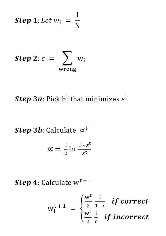
Iteratively means that Adaptive Boosting performs multiple rounds of step 2 to 4 and in the end combines all chosen classifiers in an overall formular (i.e. the strong classifier):
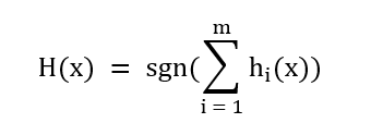
Note: The signum function is used to get an end value between -1 and +1.
So far so good, let´s have just a quick look at the model setting, on which the calculations are based!
Model Settings
For the following demonstrations, I will use the subsequent data:
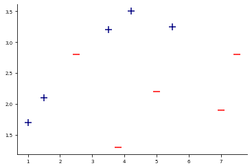
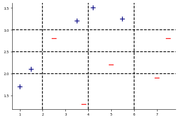
The data consists of two classes (the blue plus-signs and the red minus-signs). The goal is to correctly divide the two classes in an optimzed way. Thus, we face a Binary Classification Problem.
However, we will use the following Decision Tree Stumps
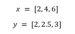
and try to find those weak classifiers (i.e. Decision Tree Stumps), which are able to correctly divide these datapoints (note that I randomly chose the Decision Tree Stumps).
Let´s visualize the final model settings on which we will perform Adaptive Boosting:
Gradually Performing Adaptive Boosting
For the first round of performing the steps, I will explain each step in detail. Afterwards, we will only look at the results of each round and see how things will change!

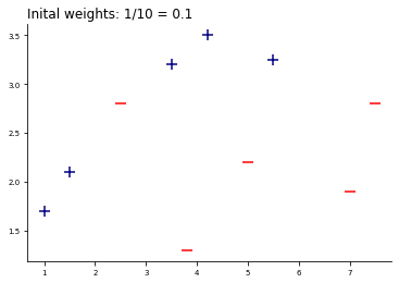
In Step 1 each data point has the same weight 1/N.
This is done, because there is no reason why we should give different weights at the beginning. Since we have 10 datapoints, the initial weights are 1/10 and hence, 0.1.
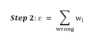
In Step 2 we draw the first Decision Tree Stump and calculate the error.
The error is used for two things: First, we need the error of each Decision Tree Stump in order to pick the Stump that has the lowest error rate (Step 3a). Second, we use the errors to calcualte the new weights (Step 4).
Weighted errors are able to focus on those datapoints, which are harder to predict. In other words, we give higher weights on those parts where prior classifiers perform badly.
Let´s see the error for the first Decision Tree Stump y = 2:
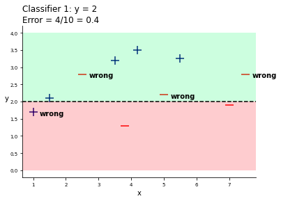
If you can see, we misclassified four data points, which leads to an error of 0.4 (4/10). This process should be done with all the chosen classifiers above. So let´s do it!
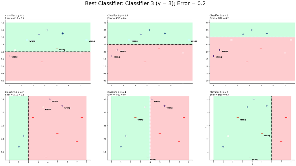
We can see all classifiers and their respective errors.

According to Step 3a, we have to pick the classifier that minimizes error. In our case, classifier 3 has the lowest error rate with 0.2.
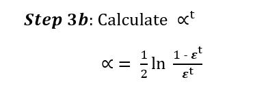
In Step 3b, we have to calculate alpha.
Alpha is used for demonstrating the voting power of a chosen classifier. The lower the error, the higher the voting power. This is useful, because more accurate classifiers should also have a higher voting power.
Note: The formular uses log, because if we would have a very small error, then alpha would get pretty high.
We will use Python to calculate alpha.
import math
def get_alpha(error):
    return (1/2)*math.log(((1-error)/error), math.e)
print("Alpha value: " + str(get_alpha(error=0.2)))
Alpha value: 0.6931471805599453
So, we have a voting power of ~0.69 for our first classifer.
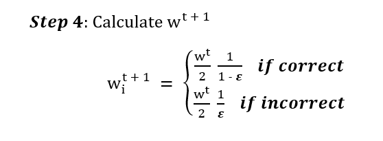
In Step 4, we need to calculate the new weights.
The new weights are calculcated at the end of each round and used to identify datapoints that are hard to classify. Once again, we use Python to calculate the new weights.
def new_weight_correct(error):
    return 0.1/(2*(1-error))
def new_weight_incorrect(error):
    return 0.1/(2*error)
print("Weights for correct classified datapoints: " + str(new_weight_correct(0.2)))
print("Weights for incorrect classified datapoints: " + str(new_weight_incorrect(0.2)))
Weights for correct classified datapoints: 0.0625
Weights for incorrect classified datapoints: 0.25
If one might notice, the datapoints, which are classified incorrectly have a higher weight (0.25) than those classified correctly (0.0625). This higher weight can be seen in the next round by looking at the sizes of the data points (I made the sizes of the datapoints in proportion to each other´s weights).
So, closing round 1, we have our first classifier (classifier 3) in the Boosting algorithm, his respective voting power and the new weights.
At the end of each round, we can reflect, if there are already enough weak classifiers to separate all data points correctly. Obviously, one round isn´t enough, so we perform round 2 with the new weights!
Since the calculations are the same for each round, I will only interpret the results from this point.

After round 2, classifier 4 is the one that minimizes the error. Note, that classifier 6 has also the same error rate, but we will choose the first one for now. However, we will continue by calculating alpha of classifier 4 and the new weights.
print("Alpha value: " + str(get_alpha(error=0.1875)))
print("Weights for correct classified datapoints: " + str(new_weight_correct(error=0.1875)))
print("Weights for incorrect classified datapoints: " + str(new_weight_incorrect(error=0.1875)))
Alpha value: 0.7331685343967135
Weights for correct classified datapoints: 0.06153846153846154
Weights for incorrect classified datapoints: 0.26666666666666666
So far so good, let´s move on with round 3:
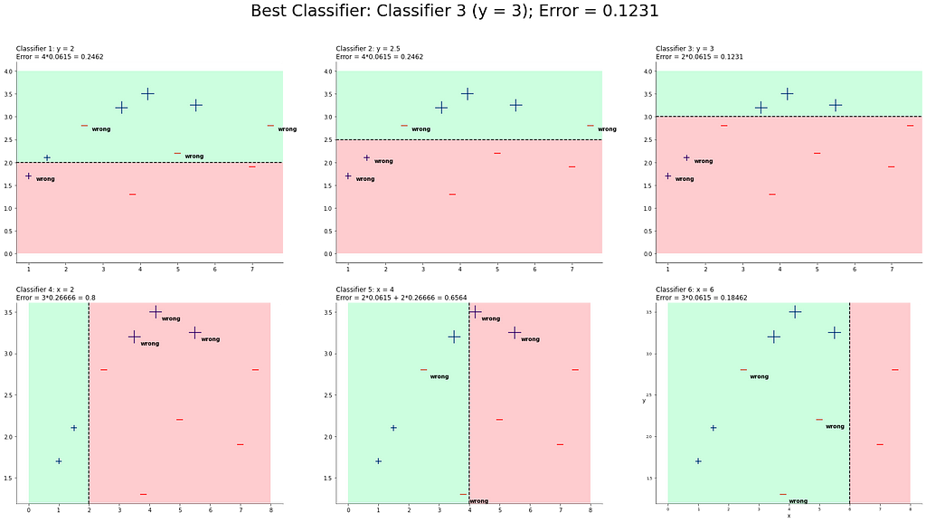
Seems that classifier 3 again is the best one. Let´s add it and calculate alpha, the new weights and start with round 4:
print("Alpha value: " + str(get_alpha(error=0.1231)))
print("Weights for correct classified datapoints: " + str(new_weight_correct(error=0.1231)))
print("Weights for incorrect classified datapoints: " + str(new_weight_incorrect(error=0.1231)))
Alpha value: 0.9816979637974511
Weights for correct classified datapoints: 0.05701904436081651
Weights for incorrect classified datapoints: 0.4061738424045492

Well, again, classifier 4 and 6 are the best. This time, we pick classifier 6!
print("Alpha value: " + str(get_alpha(error=0.1711)))
print("Weights for correct classified datapoints: " + str(new_weight_correct(error=0.1711)))
print("Weights for incorrect classified datapoints: " + str(new_weight_incorrect(error=0.1711)))
Alpha value: 0.7889256698496664
Weights for correct classified datapoints: 0.06032090722644469
Weights for incorrect classified datapoints: 0.29222676797194624
Now wait! It seems that we are at a point where we could classify all data points if we combine the classifiers. Let´s look at the end classification:
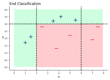
There it is! We classified everything right! Let´s try to add a new data point and let the classifiers vote!
x = 7
y = 3.5
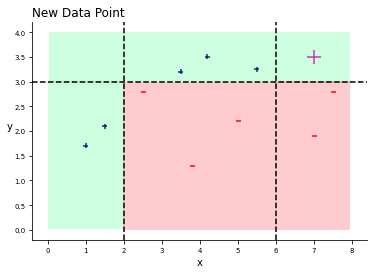
According to the final model, we have the following algorithm:

- Classifier 1 votes for plus with a voting power of 0.6931
- Classifier 2 votes for minus with a voting power of 0.7332
- Classifier 3 votes for plus with a voting power of 0.9816
- Classifier 4 votes for minus with a voting power of 0.7889.
If you calculate the weighted sum of the the voting powers, the algorithm will classify the data point as plus and guess…the algorithm is totally right!
Adaptive Boosting in Python
To show you how to implement Adaptive Boosting in Python, I use the quick example from scikit-learn, where they classify digit images based on Support Vector Machines. You can find the example and the respective code here:
Recognizing hand-written digits - scikit-learn 0.24.2 documentation
But in contrast of this example, we will classify the digits with AdaBoost. Afterwards, we will look at the performance.
Note that within AdaBoost, the default classifier is the Decision Tree Classifier. If you want other base estimators, you have to clarify them in the model.
# Importing the libraries
import matplotlib.pyplot as plt
from sklearn import datasets, metrics
from sklearn.model_selection import train_test_split
from sklearn.tree import DecisionTreeClassifier
from sklearn.ensemble import AdaBoostClassifier
digits = datasets.load_digits()
_, axes = plt.subplots(nrows=1, ncols=4, figsize=(10, 3))
for ax, image, label in zip(axes, digits.images, digits.target):
    ax.set_axis_off()
    ax.imshow(image, cmap=plt.cm.gray_r, interpolation='nearest')
    ax.set_title('Training: %i' % label)

# flatten the images
n_samples = len(digits.images)
data = digits.images.reshape((n_samples, -1))
# Split data into 50% train and 50% test subsets
X_train, X_test, y_train, y_test = train_test_split(
    data, digits.target, test_size=0.5, shuffle=False)
Alright, we are now ready to start with the AdaBoost Classifier. We will use the accuracy_score metric to define the classifier´s performance.
clf = AdaBoostClassifier()
clf.fit(X_train, y_train)
y_pred = clf.predict(X_test)
acc_sc = metrics.accuracy_score(y_test, y_pred)
print("Accuracy Score: " + str(acc_sc))
Accuracy Score: 0.7808676307007787
There it is! We are able to classify digits with and accuracy of ~78%. Note, that we did not perform hyperparameter optimzation and also used 50% as testsize(which is quite high)…so, the model could be further improved!
I hope you enjoyed this article and if you do so….then smash some claps :) Happy coding!
Adaptive Boosting: A stepwise Explanation of the Algorithm was originally published in Towards Data Science on Medium, where people are continuing the conversation by highlighting and responding to this story.
from Towards Data Science - Medium
https://towardsdatascience.com/adaptive-boosting-a-stepwise-explanation-of-the-algorithm-50b75c3729c1?source=rss----7f60cf5620c9---4
via RiYo Analytics

No comments