https://ift.tt/u1pieGf Threshold Autoregressive Models — beyond ARIMA + R Code Meet TAR — a nonlinear extension of the autoregressive mode...
Threshold Autoregressive Models — beyond ARIMA + R Code
Meet TAR — a nonlinear extension of the autoregressive model.

Introduction
When it comes to time series analysis, academically you will most likely start with Autoregressive models, then expand to Autoregressive Moving Average models, and then expand it to integration making it ARIMA. The next steps are usually types of seasonality analysis, containing additional endogenous and exogenous variables (ARDL, VAR) eventually facing cointegration. And from this moment on things start getting really interesting.
That’s because it’s the end of strict and beautiful procedures as in e.g. Box-Jenkins methodology. As explained before, the possible number of permutations of nonlinearities in time series is nearly infinite — so universal procedures don’t hold anymore. Does it mean that the game is over? Hell, no! Today, the most popular approach to dealing with nonlinear time series is using machine learning and deep learning techniques — since we don’t know the true relationship between the moment t-1 and t, we will use an algorithm that doesn’t assume types of dependency.
How did econometricians manage this problem before machine learning? That’s where the TAR model comes in.
Threshold Autoregressive Models
Let us begin with the simple AR model. Its formula is determined as:
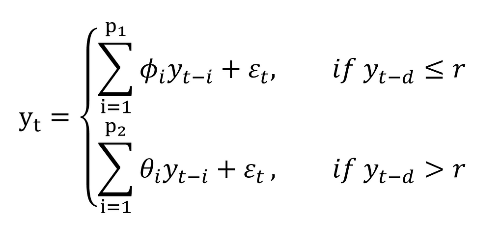
Everything is in only one equation — beautiful. Before we move on to the analytical formula of TAR, I need to tell you about how it actually works. First of all, in TAR models there’s something we call regimes. What are they? They are regions separated by the thresholds according to which we switch the AR equations. We switch, what? Let’s consider the simplest two-regime TAR model for simplicity:
Where:
p1, p2 — the order of autoregressive sub-equations,
r — the known threshold value,
Z_t — the known value in the moment t on which depends the regime
Let’s read this formula now so that we understand it better:
The value of the time series in the moment t is equal to the output of the autoregressive model, which fulfils the condition: Z ≤ r or Z > r.
Sounds kind of abstract, right? No wonder — the TAR model is a generalisation of threshold switching models. It means you’re the most flexible when it comes to modelling the conditions, under which the regime-switching takes place. I recommend you read this part again once you read the whole article — I promise it will be more clear then. Now, let’s move to a more practical example.
If we put the previous values of the time series in place of the Z_t value, a TAR model becomes a Self-Exciting Threshold Autoregressive model — SETAR(k, p1, …, pn), where k is the number of regimes in the model and p is the order of every autoregressive component consecutively. A two-regimes SETAR(2, p1, p2) model can be described by:
Now it seems a bit more earthbound, right? Let’s visualise it with a scatter plot so that you get the intuition:
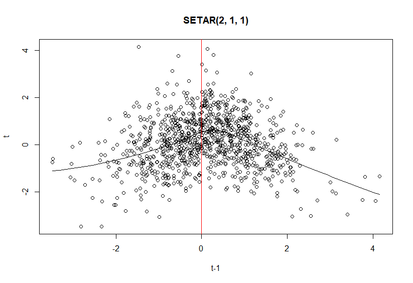
In this case, k = 2, r = 0, p1 = p2 = 1 and d = 1. You can clearly see the threshold where the regime-switching takes place. How does it look on the actual time series though?
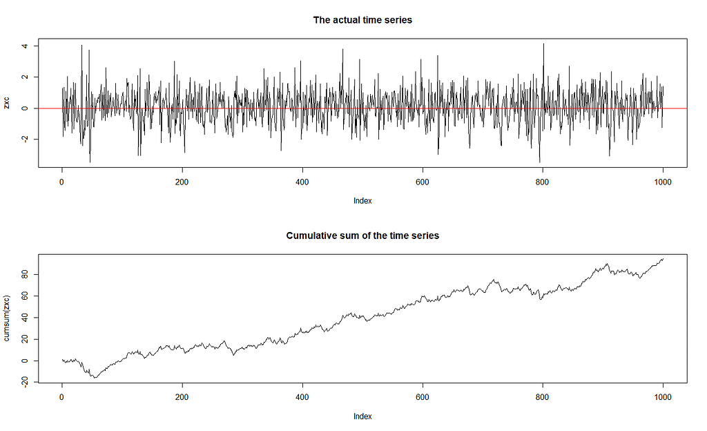
As you can see, it’s very difficult to say just from the look that we’re dealing with a threshold time series just from the look of it. What can we do then? Let’s solve an example that is not generated so that you can repeat the whole procedure.
Modelling procedure
Let’s just start coding, I will explain the procedure along the way. We are going to use the Lynx dataset and divide it into training and testing sets (we are going to do forecasting):
library("quantmod")
library("tsDyn")
library("stats")
library("nonlinearTseries")
library("datasets")
library("NTS")

data <- log10(datasets::lynx)

train <- data[1:80]
test <- data[81:114]
I logged the whole dataset, so we can get better statistical properties of the whole dataset. Now, let’s check the autocorrelation and partial autocorrelation:
{par(mfrow=c(2,1))
acf(train)
pacf(train)}
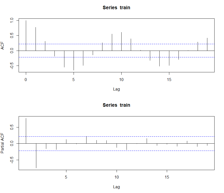
It seems like this series is possible to be modelled with ARIMA — will try it on the way as well. Nevertheless, let’s take a look at the lag plots:
{par(mfrow=c(2,2))
  scatter.smooth(Lag(train, 1), train, span = 2/3, degree = 1,
                 family = c("symmetric", "gaussian"), evaluation = 50,
  xlab = "t-1", ylab = "t")
  scatter.smooth(Lag(train, 2), train, span = 2/3, degree = 1,
                 family = c("symmetric", "gaussian"), evaluation = 50,
  xlab = "t-2", ylab = "t")
  scatter.smooth(Lag(train, 3), train, span = 2/3, degree = 1,
                 family = c("symmetric", "gaussian"), evaluation = 50,
  xlab = "t-3", ylab = "t")
  scatter.smooth(Lag(train, 4), train, span = 2/3, degree = 1,
                 family = c("symmetric", "gaussian"), evaluation = 50,
  xlab = "t-4", ylab = "t")
}
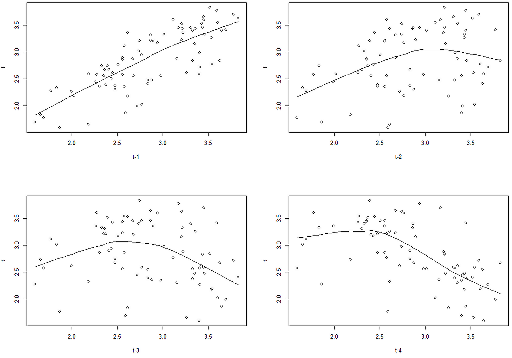
In the first lag, the relationship does seem fit for ARIMA, but from the second lag on nonlinear relationship is obvious. Sometimes however it happens so, that it’s not that simple to decide whether this type of nonlinearity is present. In this case, we’d have to run a statistical test — this approach is the most recommended by both Hansen’s and Tsay’s procedures. In order to do it, however, it’s good to first establish what lag order we are more or less talking about. We will use Average Mutual Information for this, and we will limit the order to its first local minimum:
mutualInformation(train)
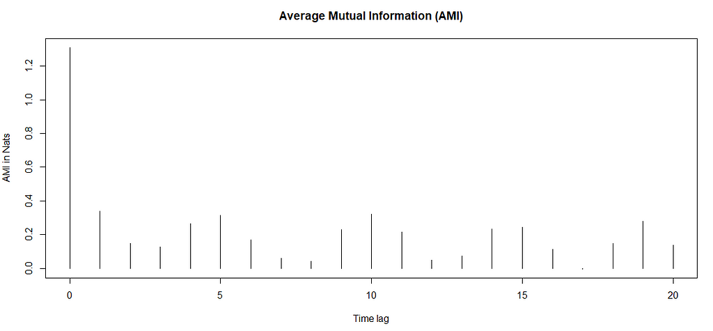
Thus, the embedding dimension is set to m=3. Of course, this is only one way of doing this, you can do it differently. Note, that again we can see strong seasonality. Now, that we’ve established the maximum lag, let’s perform the statistical test. We are going to use the Likelihood Ratio test for threshold nonlinearity. Its hypotheses are:
H0: The process is an AR(p)
H1: The process is a SETAR(p, d)
This means we want to reject the null hypothesis about the process being an AR(p) — but remember that the process should be autocorrelated — otherwise, the H0 might not make much sense.
for (d in 1:3){
  for (p in 1:3){
    cat("p = ", p, " d = ", d, " P-value = ", thr.test(train, p=p, d=d), "\n")
  }
}
SETAR model is entertained
Threshold nonlinearity test for (p,d):  1 1
F-ratio and p-value:  0.5212731 0.59806

SETAR model is entertained
Threshold nonlinearity test for (p,d):  2 1
F-ratio and p-value:  2.240426 0.1007763

SETAR model is entertained
Threshold nonlinearity test for (p,d):  3 1
F-ratio and p-value:  1.978699 0.1207424

SETAR model is entertained
Threshold nonlinearity test for (p,d):  1 2
F-ratio and p-value:  37.44167 1.606391e-09

SETAR model is entertained
Threshold nonlinearity test for (p,d):  2 2
F-ratio and p-value:  8.234537 0.0002808383

SETAR model is entertained
Threshold nonlinearity test for (p,d):  3 2
F-ratio and p-value:  7.063951 0.0003181314

SETAR model is entertained
Threshold nonlinearity test for (p,d):  1 3
F-ratio and p-value:  30.72234 1.978433e-08

SETAR model is entertained
Threshold nonlinearity test for (p,d):  2 3
F-ratio and p-value:  3.369506 0.02961576

SETAR model is entertained
Threshold nonlinearity test for (p,d):  3 3
F-ratio and p-value:  3.842919 0.01135399
As you can see, at alpha = 0.05 we cannot reject the null hypothesis only with parameters d = 1, but if you come back to look at the lag plots you will understand why it happened.
Another test that you can run is Hansen’s linearity test. Its hypotheses are:
H0: The time series follows some AR process
H1: The time series does not follow some SETAR process
This time, however, the hypotheses are specified a little bit better — we can test AR vs. SETAR(2), AR vs. SETAR(3) and even SETAR(2) vs SETAR(3)! Let’s test our dataset then:
setarTest(train, m=3, nboot=400)
setarTest(train, m=3, nboot=400, test='2vs3')
Test of linearity against setar(2) and setar(3)

         Test   Pval
1vs2 25.98480 0.0175
1vs3 46.31897 0.0150


Test of setar(2) against  setar(3)

         Test   Pval
2vs3 15.20351 0.2425
This test is based on the bootstrap distribution, therefore the computations might get a little slow — don’t give up, your computer didn’t die, it needs time :) In the first case, we can reject both nulls — the time series follows either SETAR(2) or SETAR(3). From the second test, we figure out we cannot reject the null of SETAR(2) — therefore there is no basis to suspect the existence of SETAR(3). Therefore SETAR(2, p1, p2) is the model to be estimated.
So far we have estimated possible ranges for m, d and the value of k. What is still necessary is the threshold value r. Unfortunately, its estimation is the most tricky one and has been a real pain in the neck of econometricians for decades. I do not know about any analytical way of computing it (if you do, let me know in the comments!), instead, usually, grid-search is performed.
The intuition behind is a little bit similar to Recursive Binary Splitting in decision trees — we estimate models continuously with an increasing threshold value. Fortunately, we don’t have to code it from 0, that feature is available in R. Before we do it however I’m going to explain shortly what you should pay attention to.
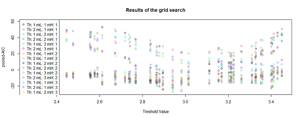
We want to achieve the smallest possible information criterion value for the given threshold value. Nevertheless, this methodology will always give you some output! What you are looking for is a clear minimum. This is what would look good:
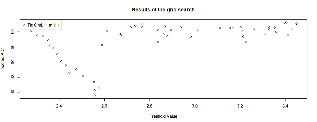
There is a clear minimum a little bit below 2.6. The more V-shaped the chart is, the better — but it’s not like you will always get a beautiful result, therefore the interpretation and lag plots are crucial for your inference. This is what does not look good:
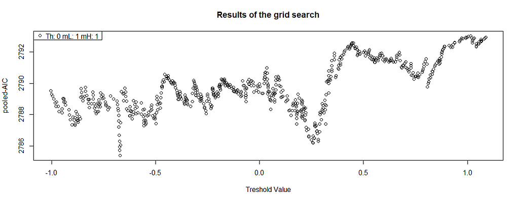
Whereas this one also has some local minima, it’s not as apparent as it was before — letting SETAR take this threshold you’re risking overfitting. In practice though it never looks so nice — you’re searching for many combinations, therefore there will be many lines like this. Let’s get back to our example:
selectSETAR(train, m=3, thDelay=1:2)
Using maximum autoregressive order for low regime: mL = 3
Using maximum autoregressive order for high regime: mH = 3
Searching on 50 possible threshold values within regimes with sufficient ( 15% ) number of observations
Searching on  900  combinations of thresholds ( 50 ), thDelay ( 2 ), mL ( 3 ) and MM ( 3 )
Results of the grid search for 1 threshold
   thDelay mL mH       th pooled-AIC
1        2  3  3 2.940018  -26.88059
2        2  3  3 2.980912  -26.44335
3        2  3  2 2.940018  -24.66521
4        2  3  2 2.980912  -24.43568
5        2  3  3 2.894316  -24.20612
6        2  3  3 3.399847  -22.98202
7        2  3  2 2.894316  -22.89391
8        2  2  3 2.940018  -22.15513
9        2  3  2 3.399847  -21.34704
10       2  1  3 2.940018  -20.52942
Therefore the preferred coefficients are:
thDelay mL mH       th pooled-AIC
2        3  3 2.940018  -26.88059
Great! It’s time for the final model estimation:
model <- setar(train, m=3, thDelay = 2, th=2.940018)
summary(model)
Non linear autoregressive model

SETAR model ( 2 regimes)
Coefficients:
Low regime:
   const.L     phiL.1     phiL.2     phiL.3
 0.8765919  0.9752136  0.0209953 -0.2520500

High regime:
   const.H     phiH.1     phiH.2     phiH.3
 0.3115240  1.6467881 -1.3961317  0.5914694

Threshold:
-Variable: Z(t) = + (0) X(t)+ (0)X(t-1)+ (1)X(t-2)
-Value: 2.94 (fixed)
Proportion of points in low regime: 55.84%   High regime: 44.16%

Residuals:
       Min         1Q     Median         3Q        Max
-0.5291117 -0.1243479 -0.0062972  0.1211793  0.4866163

Fit:
residuals variance = 0.03438,  AIC = -254, MAPE = 5.724%

Coefficient(s):

         Estimate  Std. Error  t value  Pr(>|t|)
const.L  0.876592    0.227234   3.8577 0.0002469 ***
phiL.1   0.975214    0.142437   6.8466 2.117e-09 ***
phiL.2   0.020995    0.196830   0.1067 0.9153498
phiL.3  -0.252050    0.121473  -2.0749 0.0415656 *
const.H  0.311524    0.685169   0.4547 0.6507163
phiH.1   1.646788    0.172511   9.5460 2.027e-14 ***
phiH.2  -1.396132    0.277983  -5.0224 3.576e-06 ***
phiH.3   0.591469    0.272729   2.1687 0.0334088 *
---
Signif. codes:  0 ‘***’ 0.001 ‘**’ 0.01 ‘*’ 0.05 ‘.’ 0.1 ‘ ’ 1

Threshold
Variable: Z(t) = + (0) X(t) + (0) X(t-1)+ (1) X(t-2)

Value: 2.94 (fixed)
SETAR model has been fitted. Now, since we’re doing forecasting, let’s compare it to an ARIMA model (fit by auto-arima):
ARIMA(4,0,1) with non-zero mean

Coefficients:
         ar1     ar2      ar3      ar4     ma1    mean
      0.3636  0.4636  -0.4436  -0.2812  0.9334  2.8461
s.e.  0.1147  0.1290   0.1197   0.1081  0.0596  0.0515

sigma^2 = 0.0484:  log likelihood = 8.97
AIC=-3.93   AICc=-2.38   BIC=12.74

Training set error measures:
                        ME      RMSE       MAE        MPE     MAPE      MASE
Training set -0.0002735047 0.2115859 0.1732282 -0.6736612 6.513606 0.5642003
                     ACF1
Training set -0.002296863
SETAR seems to fit way better on the training set. Now let’s compare the results with MSE and RMSE for the testing set:
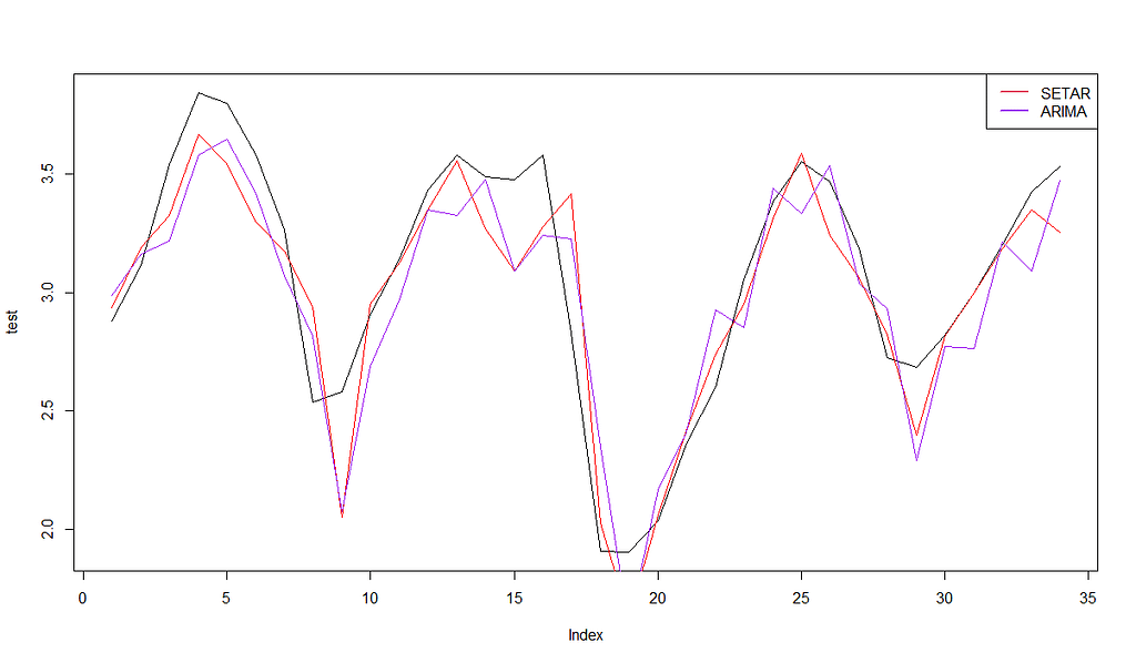
SETAR MSE: 0.04988592
SETAR RMSE: 0.2233516

ARIMA MSE: 0.06146426
ARIMA RMSE: 0.2479199
As you can see, SETAR was able to give better results for both training and testing sets.
Final notes
- Stationarity of TAR — this is a very complex topic and I strongly advise you to look for information about it in scientific sources. Nevertheless, there is an incomplete rule you can apply: If there is a unit root in any of the regimes, the whole process is nonstationary.
- The first generated model was stationary, but TAR can model also nonstationary time series under some conditions. It’s safe to do it when its regimes are all stationary. In this case, you will most likely be dealing with structural change.
- The number of regimes — in theory, the number of regimes is not limited anyhow, however from my experience I can tell you that if the number of regimes exceeds 2 it’s usually better to use machine learning.
- SETAR model is very often confused with TAR — don’t be surprised if you see a TAR model in a statistical package that is actually a SETAR. Every SETAR is a TAR, but not every TAR is a SETAR.
- To fit the models I used AIC and pooled-AIC (for SETAR). If your case requires different measures, you can easily change the information criteria.
Summary
Threshold Autoregressive models used to be the most popular nonlinear models in the past, but today substituted mostly with machine learning algorithms. Nonetheless, they have proven useful for many years and since you always choose the tool for the task, I hope you will find it useful.
Of course, SETAR is a basic model that can be extended. If you are interested in getting even better results, make sure you follow my profile!
You can also reach me on LinkedIn.
Link to the data (GNU).
Nonlinear Time Series — an intuitive introduction
Threshold Autoregressive Models — beyond ARIMA + R code was originally published in Towards Data Science on Medium, where people are continuing the conversation by highlighting and responding to this story.
from Towards Data Science - Medium
https://towardsdatascience.com/threshold-autoregressive-models-beyond-arima-r-code-6af3331e2755?source=rss----7f60cf5620c9---4
via RiYo Analytics


No comments